Maximum Likelihood Estimation
Estimating distribution parameters from an observed sample is a general problem in most scenarios, termed parameter estimation problems. Given the observed data $X=(x_1,x_2,\dots,x_n)$ satisfying i.i.d. assumption, our goal is to determine the most likely parameters describing the distribution of $X$. The likelihood is a function of $\theta$ as
\[L(\theta)=p(X\vert\theta)=\prod_{i=1}^np(x_i\vert\theta),\]which describes the chance that each possible parameter value produced the data we observed. Intuitively, the most likely parameters correspond to the maximum likelihood function. Assuming that $X$ follows Gaussian distribution where $\theta=(\mu,\sigma^2)$, we can easily estimate them via a bit of calculus and derivatives as
\[\hat{\theta}=\arg\max_\theta\prod_{i=1}^np(x_i\vert\theta)=\arg\max_{\mu,\sigma^2}\prod_{i=1}^n\frac{1}{\sqrt{2\pi\sigma^2}}\exp(-\frac{(x_i-\mu)^2}{2\sigma^2}),\] \[\frac{\partial\log L}{\partial\mu}=0\Rightarrow\mu=\frac{1}{n}\sum_{i=1}^nx_i,\] \[\frac{\partial\log L}{\partial\sigma^2}=0\Rightarrow\sigma^2=\frac{1}{n}\sum_{i=1}^n(x_i-\mu)^2.\]To simplify the calculation process, it is common to apply the logarithm to the likelihood function, resulting in the log-likelihood function. This approach is sometimes referred to as log-likelihood estimation. The maximum likelihood estimates (MLEs) obtained from the log-likelihood function represent fixed values for the estimated distribution parameters. Therefore, MLE is a type of point estimation.
Likelihood to Loss function
The intriguing core of MLE is transforming an estimation problem into an optimization one which can be efficiently solved via gradient descent methods. For example, an autoencoder represented by $f_\theta$ can be used to reconstruct the input as $x\xrightarrow{f_\theta}\hat{x}$. In practice, the distance between $x$ and $\hat{x}$ is measured by the p-norm as
\[L(\theta)=\mathbb{E}_{x\sim p(x)}\Vert x-\hat{x}\Vert_p\approx\frac{1}{n}\sum_{i=1}^n\Vert x_i-\hat{x}_i\Vert_p,\]where we can obtain the optimal $\theta$ by minimizing above loss function. When $p=2$ and omitting the squared root operation, the loss function is simply the mean squared error (MSE). We can also view the input data $X$ as a random variable. Assuming the true distribution of the data is Gaussian, the probability and the log-likelihood of the observed input $x$ is
\[p(x\vert\mu,\sigma^2)=\frac{1}{\sqrt{2\pi\sigma^2}}\exp({-\frac{(x - \mu)^2}{2\sigma^2}}),\] \[\log p(x\vert\mu,\sigma^2)=-\frac{1}{2}\log(2\pi\sigma^2)-\frac{(x-\mu)^2}{2\sigma^2}.\]Maximizing this log-likelihood is equivalent to minimizing the negative log-likelihood, which corresponds to the MSE loss function as
\[-\log p(x\vert\mu,\sigma^2) \propto \text{MSE} = \frac{1}{n} \sum_{i=1}^{n} (\hat{x}_i-x_i)^2,\] \[\arg\max_\theta \log p(X\vert\theta)=\arg\min_\theta\Vert f_\theta(X)-X\Vert^2.\]When $p=2$, the loss function of the autoencoder can be interpreted as a maximum likelihood estimation problem, where we assume a Gaussian distribution for the input data. (1-norm corresponds to Laplace distribution)
Bayesian Estimation
Bayesian Estimation derives from Bayes’ Theorem given by
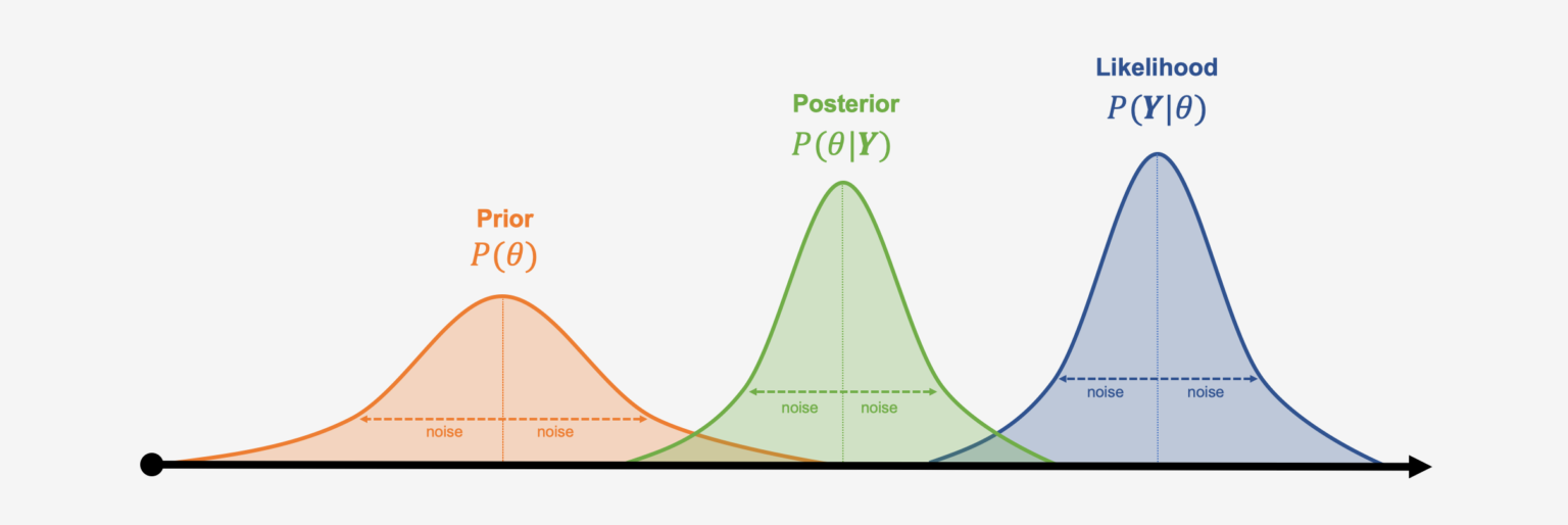
\[\underbrace{p(\theta\vert X)}_{\text{posterior}}=\frac{\overbrace{p(X\vert\theta)}^{\text{likelihood}}\cdot \overbrace{p(\theta)}^{\text{prior}}}{\underbrace{\int p(X\vert\theta)\cdot p(\theta)\text{d}\theta}_{\text{evidence}}},\]where we update the prior beliefs $p(\theta)$ based on new observations $X$. Different from MLEs, Bayesian approach treats $\theta$ as a random variable taking values in parameter space $\Theta$. However, it is hard to compute the integral in the denominator due to the large parameter space. This is why the posterior distribution is often deemed to be intractable. Here we will introduce two methods to deal with intractable problem.
Maximum a Posteriori (MAP) Estimation
Considering that the denominator $p(X)$ is independent of the parameter $\theta$ to be estimated, we can get $p(\theta\vert X)\propto p(X\vert\theta)\cdot p(\theta)$. Thus,
\[\arg\max_\theta p(X\vert\theta)=\arg\max_\theta p(X\vert\theta)\cdot p(\theta).\]It is similar to MLE, yet we introduce the prior knowledge $p(\theta)$ to narrow the parameter space. MLE is a special MAP estimation where the prior is the uniform distribution.
Variational Bayes Inference
A more general approach to solving intractable problem is variational inference. Supposing we have a tractable distribution $q(\theta)$, we can make $q(\theta)$ and $p(\theta\vert X)$ ‘close’ to estimate $\theta$. Considering the KL divergence between $q$ and $p$, we have
\[\text{KL}(q\Vert p)=\int q(\theta)\log\frac{q(\theta)}{p(\theta\vert X)}\text{d}\theta=\mathbb{E}_q\log\frac{q(\theta)}{p(\theta\vert X)},\] \[\log p(\theta\vert X)=\log p(X\vert\theta)+\log p(\theta)-\log p(X),\] \[\log p(x)=\text{KL}(q\Vert p)+\mathbb{E}_q\log\frac{p(x,\theta)}{q(\theta)}.\]Because KL divergence is strictly non-negative, the second term is a lower bound for $\log p(x)$, also known as the evidence lower bound (ELBO). Minimizing the KL divergence between $q$ and $p$ is equivalent to maximizing the second term. See VAE for more details on calculating the ELBO via the reparameterization trick.
Expectation-Maximization Algorithm
In some cases, the observation $X$ may be incomplete or accompanied by the influence of latent variables $Z$ as
\[\hat{\theta}=\arg\max_\theta\log p(X\vert\theta)=\arg\max_\theta\log\sum_Zp(X,Z\vert\theta),\]where we can’t directly perform maximum likelihood estimation due to the sum within the logarithm. Fortunately, we can extract the sum operation from the logarithm through the Jensen’s inequality
\[\begin{aligned} L(\theta) &= \log\sum_Zp(X,Z\vert\theta), \\ &= \log\mathbb{E}_{z\sim q(z)}\frac{p(X,z\vert\theta)}{q(z)}, \\ &\geq\underbrace{\mathbb{E}_{z\sim q(z)}\log\frac{p(X,z\vert\theta)}{q(z)}}_{\text{ELBO}}. \end{aligned}\]Given the condition for the equality to hold, we can get
\[\begin{cases} \sum_zq(z)=1 \\ \displaystyle\frac{p(X,z\vert\theta)}{q(z)}=\text{constant} \end{cases}\Rightarrow q(z)=p(z\vert X,\theta),\] \[\arg\max_\theta\log p(X\vert\theta)=\arg\max_\theta\mathbb{E}_{z\sim q(z)}\log p(X,z\vert\theta)\approx\arg\max_\theta\sum_x\sum_z\log p(x,z\vert\theta).\]In summary, the two steps of the EM algorithm are
- E-step: estimating the expected value of $q(z)=p(z\vert X,\theta)$ given the observed data $X$ and current parameters $\theta$;
- M-step: updating the parameters via maximizing the expectation over $\theta$.
General EM Algorithm
Let’s rethink the log-likelihood $\log p(X\vert\theta)$ with latent variables $Z$. Given the chain rule, we can easily get
\[\begin{aligned} \log p(X\vert\theta) &= \log p(X,Z\vert\theta)-\log p(Z\vert X,\theta), \\ &= \mathbb{E}_{z\sim q(z)}\log\frac{p(X,z\vert\theta)}{q(z)}-\mathbb{E}_{z\sim q(z)}\log\frac{p(z\vert X,\theta)}{q(z)}, \\ &= \underbrace{\mathbb{E}_{z\sim q(z)}\log\frac{p(X,z\vert\theta)}{q(z)}}_{\text{ELBO}}+\text{KL}(q\Vert p(z\vert X,\theta)). \end{aligned}\]Here the evidence lower bound is the same as above. The original EM algorithm sets the KL divergence term to $0$ assuming that the $q(z)=p(z\vert X,\theta)$ is tractable. GEM weakens this hypothesis, and can calculate $q(z)$ via variational inference.