From AE to VAE

PAPER
Extracting and composing robust features with denoising autoencoders
Auto-Encoding Variational Bayes
Tutorial on Variational Autoencoders

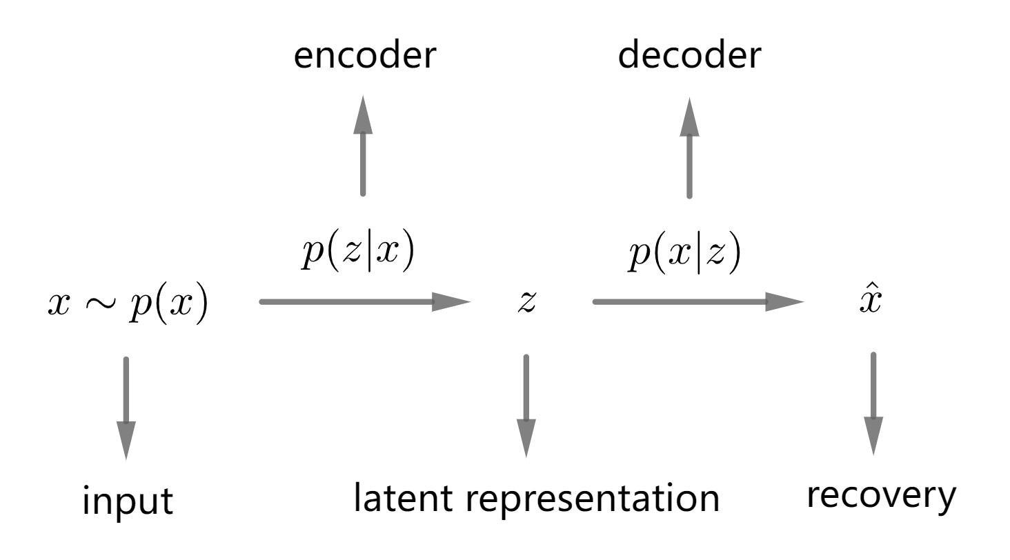
Autoencoders

Autoencoders generally contains an encoder and decoder. The encoder $f_\theta$ projects the original input $x$ into the latent representation $z$, and the decoder $g_\phi$ reconstructs the input data from $z$. That is, Autoencoders are used to learn an identical map between the input and output, which are suitable for most compression/decompression tasks.

\[x\xrightarrow{f_\theta}z\xrightarrow{g_\phi}\tilde{x}\] \[L_{\theta,\phi}=\Vert x-g_\phi(f_\theta(x))\Vert_2\]

class Autoencoders(nn.Module):
    def __init__(self, input_dim=96, hidden_states=128, z_dim=512):
        super(Autoencoders, self).__init__()
        self.encoder = nn.Sequential(
            nn.Linear(input_dim, hidden_states),
            nn.ReLU(),
            nn.Linear(hidden_states, z_dim)
        )
        
        self.decoder = nn.Sequential(
            nn.Linear(z_dim, hidden_states),
            nn.ReLU(),
            nn.Linear(hidden_states, input_dim)
        )
        
    def forward(self, x):
        # x: [batch, length, dimension]
        x = self.encoder(x)
        recon_x = self.decoder(x)

        return recon_x

Since the autoencoders learn the identity function, the overfitting problem is ubiquitous when the network scale expands. Denoising Autoencoders (DAE) are proposed to avoid overfitting via “denoising”. DAE corrupts the input $x$ (i.e. introduce the noise) and recovers the original input data to alleviate overfitting mainly caused by the noise. Specifically, in the original DAE paper, the noise is introduced by randomly setting a fixed proportion of values in input data to zero, which is similar to dropout. In practice, we can choose any type of noise such as Gaussian noise. Recently the prevailing Masked Autoencoders (MAE) are actually a special DAE which applies masking noise to the input data.

Variational Autoencoders

Different from all the autoencoders, the primary goal of Variational Autoencoders (VAE) is to learn how to generate natural data (i.e. estimate the true distribution $p(x)$ of $x$). For compression and decompression tasks, the encoder $f_\theta(z\vert x)$, decoder $g_\phi(x\vert z)$ and $z$ are accessible to each data $x$. But for generation tasks, we do not know the specific $z$ of each target $\tilde{x}$ to be generated. Thus, we should first determine the latent variables $z$.

Considering the high dimension of the raw data $x$, we should embed $x$ into latent space $z$ which can easily be sampled from $p(z)$. Assume we have a family of functions $f(z;\theta)$, where $\theta$ is learnable parameter. Optimize $\theta$ such that $f(z;\theta)$ can produce samples like $x$ with high probability.

\[\arg\max_\theta p(x)=\int p(x\vert z;\theta)\cdot p(z)\text{d}z\]

Here, $f(z;\theta)$ is replaced by $p(x\vert z;\theta)$ due to maximum likelihood. In VAEs, the choice of this output distribution is often Gaussian. You can also use other distribution but you should guarantee that $\theta$ is continuous. To optimize $p(x)$, there are two problems we should deal with:

How to define the latent variables $z$?
How to deal with the integral over $z$?

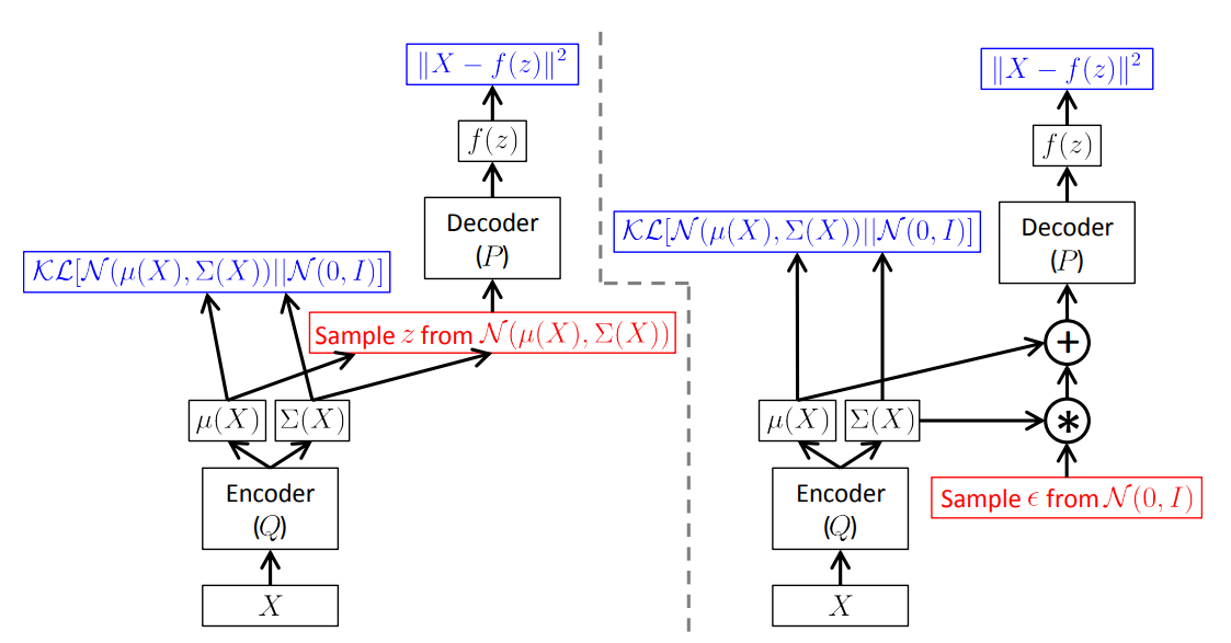
VAE assumes that there is no simple interpretation of the dimensions of $z$ and instead asserts that samples of $z$ can be drawn from a simple Gaussian distribution $p(z)\sim N(0,1)$. Then we can sample a large number of $z$ values to estimate $p(x)\approx\frac{1}{n}\sum_ip_\theta(x\vert z_i)$. However, $p_\theta(x\vert z)$ will be nearly zero for most $z$. The key idea behind VAE is to attempt to sample values of $z$ that are likely to have produced $x$, which means we need to learn a new approximation function $q_\phi(z)$ where we can get a distribution over $z$ values which are likely to produce $x$. Then we should make $q_\phi(z)$ and the true posterior distribution $p(z\vert x)$ more similar (i.e. minimize the KL divergence between them) so that we can estimate $p(x)\approx\mathbb{E}{z\sim q}p\theta(x\vert z)$.

\[KL(q(z)\Vert p(z\vert x))=\mathbb{E}_{z\sim q}[\log q(z)-\log p(z\vert x)]\] \[\log p(z\vert x)=\log p(x\vert z)+\log p(z)-\log p(x)\] \[\log p(x)-D(q(z),p(z\vert x))=\mathbb{E}_{z\sim q}\log p(x\vert z)-KL(q(z)\Vert p(z))\]

Our goal is to maximize $p(x)$ and minimize $D(q(z),p(z\vert x))$, which is equal to optimize the right hand side of the equation:

maximize the expectation of the reconstruction of data points from the latent vector
minimize the divergence between the estimated latent vector and the true latent vector

To apply SGD on the right hand side of above equation, we should specify all the terms. We know $p(z)\sim N(0,1)$ and $q$ is often initialized as Gaussian with learnable mean and variance. The expectation $\mathbb{E}_{z\sim q}\log p(x\vert z)$ can be estimated by reparameterization trick.

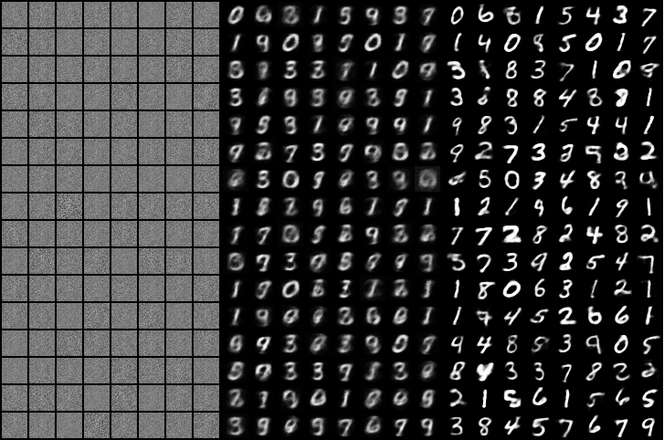
\[z=\mu+\sigma\odot\varepsilon\] \[-L_{\theta,\phi}=\mathbb{E}_{\varepsilon\sim N(0,1)}\log p_\theta(x\vert z)-KL(q_\phi(z)\Vert p_\theta(z))\leq\log p(x)\] \[\begin{aligned} KL(N(\mu,\sigma^2)\Vert N(0,1)) &= \int\frac{1}{\sqrt{2\pi\sigma^2}}e^{-(x-\mu)^2/2\sigma^2}\cdot\log\frac{e^{-(x-\mu)^2/2\sigma^2}/\sqrt{2\pi\sigma^2}}{e^{-x^2/2}/\sqrt{2\pi}}\text{d}x \\ &= \frac{1}{2}\int\frac{1}{\sqrt{2\pi\sigma^2}}e^{-(x-\mu)^2/2\sigma^2}\cdot[-\log\sigma^2+x^2-(x-\mu)^2/\sigma^2]\text{d}x \\ &= \frac{1}{2}(-\log\sigma^2+\mu^2+\sigma^2-1) \end{aligned}\]

Here is a demo VAE trained on MNIST:

class VAE(nn.Module):
    def __init__(self, image_size=784, h_dim=400, z_dim=20):
        super(VAE, self).__init__()
        
        self.encoder = nn.Sequential(
            nn.Linear(image_size, h_dim),
            nn.LeakyReLU(0.2),
            nn.Linear(h_dim, z_dim*2)
        )
        self.decoder = nn.Sequential(
            nn.Linear(z_dim, h_dim),
            nn.ReLU(),
            nn.Linear(h_dim, image_size),
            nn.Sigmoid()
        )
    
    def reparameterize(self, mu, logvar):
        std = logvar.mul(0.5).exp_().to(device)
        esp = torch.randn(*mu.size()).to(device)
        z = mu + std * esp

        return z
    
    def forward_loss(self, recon_x, x, mu, logvar):
        # BCE with sigmoid can be replaced by F.mse_loss()
        BCE = F.binary_cross_entropy(recon_x, x, reduction='sum')
        KLD = -0.5 * torch.sum(1 + logvar - mu**2 -  logvar.exp())

        return BCE + KLD

    def forward(self, x):
        # x: [batch, 784]
        h = self.encoder(x)
        # encoder: [batch, 40]
        mu, logvar = torch.chunk(h, 2, dim=1)
        # paras, z: [batch, 20]
        z = self.reparameterize(mu, logvar)
        recon_x = self.decoder(z)

        return recon_x, self.forward_loss(recon_x, x, mu, logvar)

In essence, VAE postulates that each data corresponds to a Gaussian distribution $p_\theta(z\vert x)$. Our goal is to learn a generator $q_\phi(z)$ and narrow the space of $z$ via minimizing the KL divergence between $p_\theta(z\vert x)$ and $N(0,1)$ for better sampling and generation. $-L_{\theta,\phi}$ is actually the Evidence Lower Bound (ELBO) of $\log p(x)$, which is derived from variational inference. That’s why we call it VAE.

Conditional Variational Autoencoders

To control the generation output, we can introduce the conditional context like label information to the input as $p(x\vert z,c)$. Here we provide an example of CVAE to generate the number “1”, “4” and “8” in MINST where we utilize the one-hot label as the conditional context.

class CVAE(nn.Module):
    def __init__(self, image_size, h_dim, z_dim, context_dim):
        super(CVAE, self).__init__()
        
        self.encoder = nn.Sequential(
            nn.Linear(image_size + context_dim, h_dim),
            nn.LeakyReLU(0.2),
            nn.Linear(h_dim, z_dim*2)
        )
        self.decoder = nn.Sequential(
            nn.Linear(z_dim + context_dim, h_dim),
            nn.ReLU(),
            nn.Linear(h_dim, image_size),
            nn.Sigmoid()
        )
    
    def reparameterize(self, mu, logvar):
        std = logvar.mul(0.5).exp_().to(device)
        esp = torch.randn(*mu.size()).to(device)
        z = mu + std * esp

        return z
    
    def forward_loss(self, recon_x, x, mu, logvar):
        # BCE with sigmoid can be replaced by F.mse_loss()
        BCE = F.binary_cross_entropy(recon_x, x, reduction='sum')
        KLD = -0.5 * torch.sum(1 + logvar - mu**2 -  logvar.exp())

        return BCE + KLD

    def forward(self, x, context):
        # x: [batch, 784]
        h = self.encoder(torch.cat([x, context], 1))
        mu, logvar = torch.chunk(h, 2, dim=1)
        z = self.reparameterize(mu, logvar)
        recon_x = self.decoder(torch.cat([z, context], 1))

        return recon_x, self.forward_loss(recon_x, x, mu, logvar)