Motivations
Traditional machine learning methods always focus on empirical risk minimization (ERM). Given the preditions $f(x)$ and actual targets $y$, we could minimize the average of the loss function $L$ over the joint distribution $P(x,y)$:
\[R(f)=\int L(f(x),y)\text{d}P(x,y)\]$R(f)$ is known as the expected risk. The distribution $P$ is unknown in most practical situations. Thus, we usually have access to a set of training data to approximate $P$, which is called empirical distribution. Minimizing it is known as the ERM principle.
However, the convergence of ERM is guaranteed as long as the size of the learning machine does not increase with the number of training data (few-shot). Two shortages of ERM are as follows:
- ERM allows large neural networks to memorize (instead of generalize from) the training data
- Neural networks trained with ERM change their predictions drastically when evaluated on examples just outside the training distribution (sensitive to corrupt or adversarial examples)
ERM is unable to explain or provide generalization on testing distributions that differ only slightly from the training data. Thus, we need data augmentation to describe a vicinity or neighborhood around each example in the training data.
Mixup
Mixup is a simple and data-agnostic data augmentation routine. It can be understood as the linear interpolation of samples:
\[\hat{x}=\lambda x_i+(1-\lambda)x_j\] \[\hat{y}=\lambda y_i+(1-\lambda)y_j\]Where $x_i$ and $x_j$ are raw input vectors; $y_i$ and $y_j$ are one-hot label encodings. Figure 1b shows that mixup leads to decision boundaries that transition linearly from class to class, providing a smoother estimate of uncertainty.
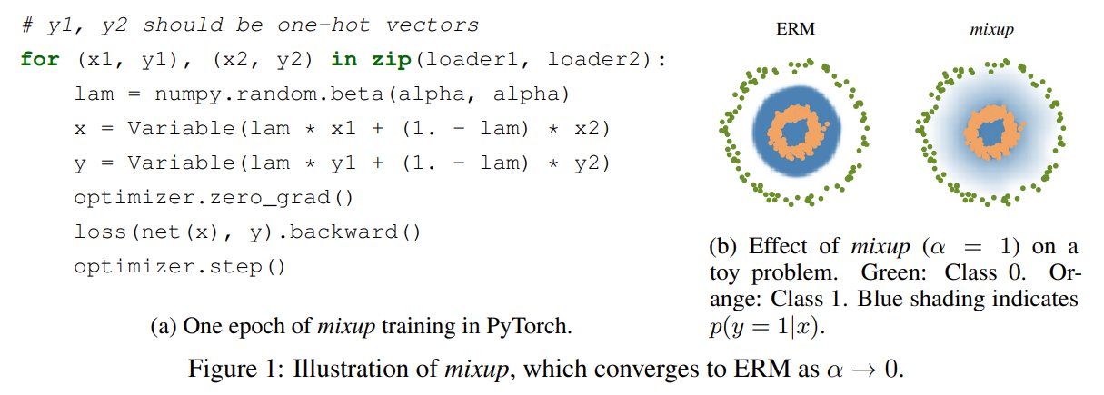
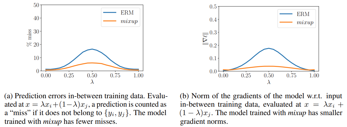
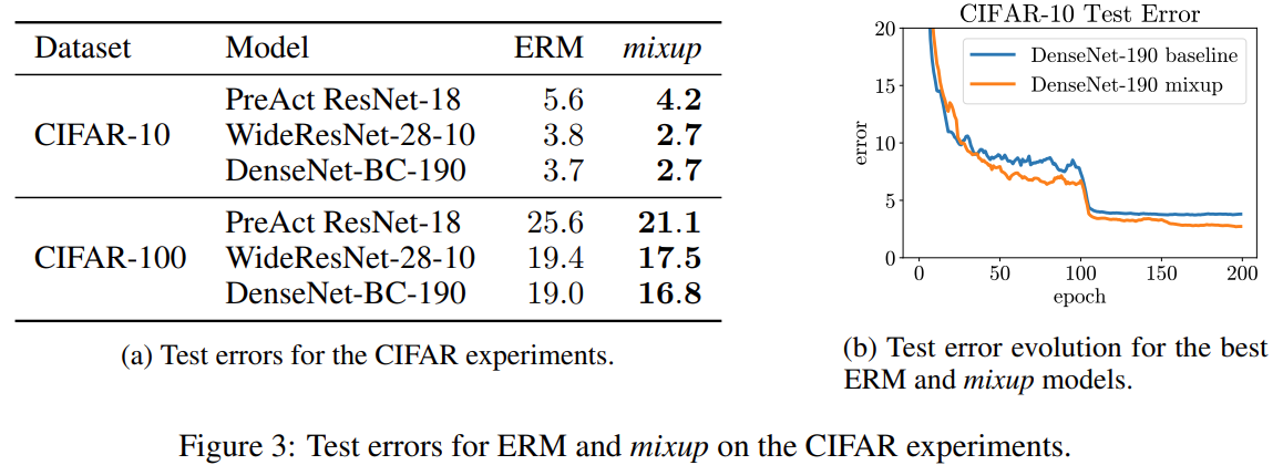
Figure 2 shows the strong robustness and generalization brought by mixup. Figure 3 shows that the models trained using mixup significantly outperform their analogues trained with ERM on the CIFAR-10 and CIFAR-100 datasets.
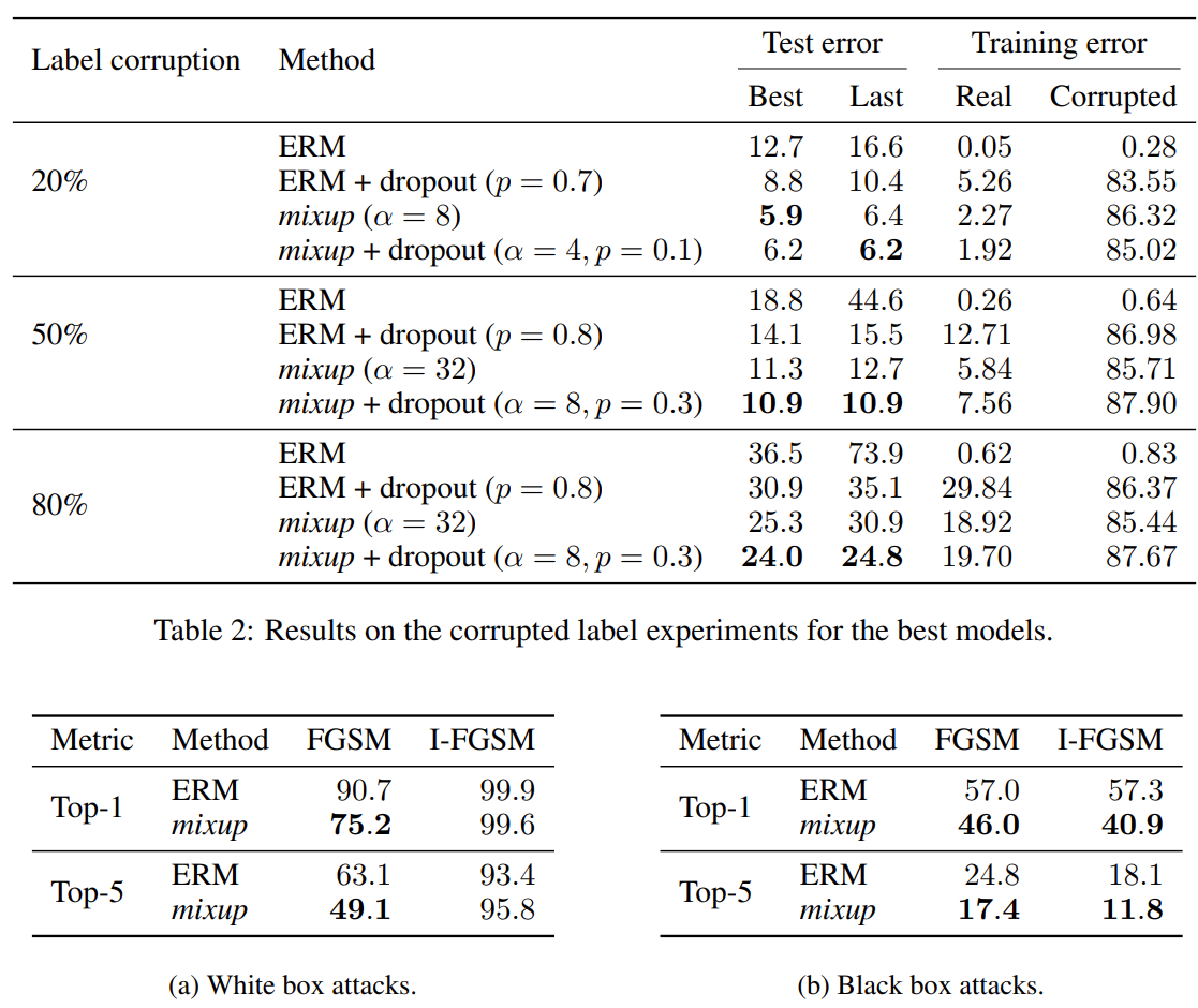
The following experiemnts show that mixup improves generalization of the model to corrupted labels (true labels are replaced by random noise). Dropout and mixup can effectively reduce overfitting.
To improve robustness of the model to adversarial examples, conventional approaches always penalize the norm of the Jacobian of the model to control its Lipschitz constant, or do data augmentation by producing and training on adversarial examples. All of these methods add significant computational overhead to ERM.
\[\max_g\min_d\mathbb{E}L(d(x),1)+L(d(g(z),0))\]Where $g(z)$ are fake samples from generator. Mixup could improve the smoothness of the discriminator, which guarantees a stable source of gradient information to the generator.
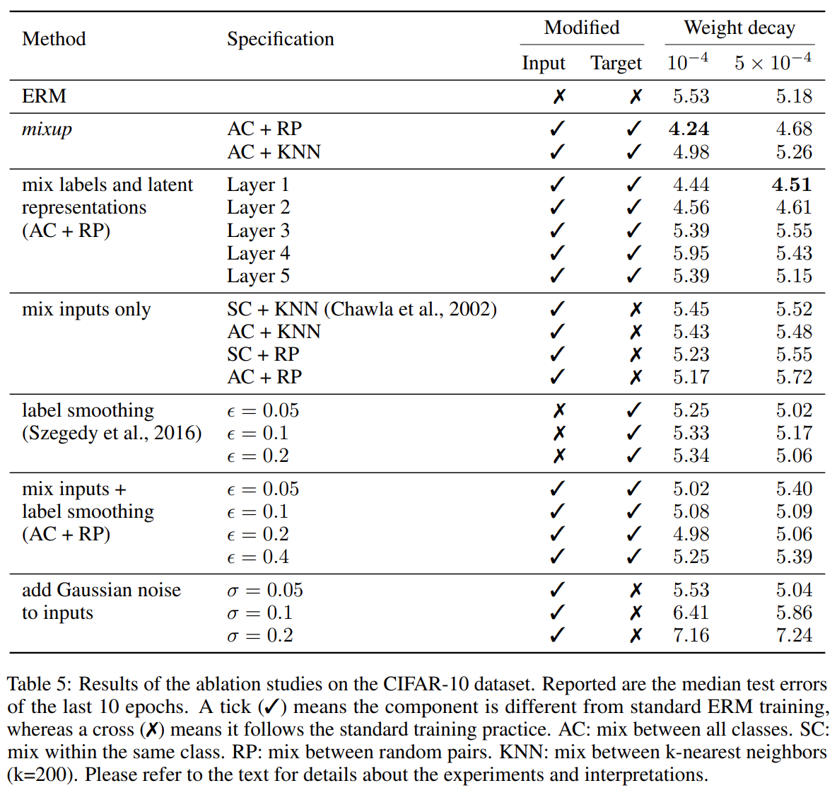
\[\max_g\min_d\mathbb{E}L(d(\lambda x+(1-\lambda)g(z)), \lambda)\]Table 5 shows the ablation study on mixup. We can see the effect of smoothness brought by mixup. They find that $\alpha\in[0.1,0.4]$ leads to improved performance over ERM. Notice that convex combinations of three or more examples with weights does not provide further gain.
To sum up, mixup is a data augmentation method that consists of only two parts: random convex combination of raw inputs, and correspondingly, convex combination of one-hot label encodings. Like other methods like label smoothing and AutoAugment, mixup improves the smoothness of the data distribution, and then enhances robustness and generalization of the model.
Extension of mixup
CutMix: patches are cut and pasted among training images where the ground truth labels are also mixed proportionally to the area of the patches.
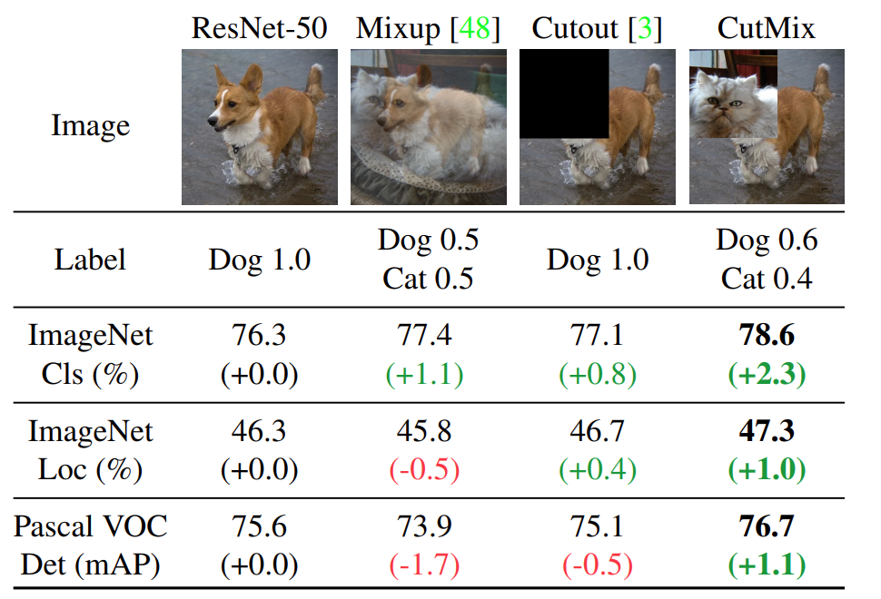
CutMix is motivated by regional dropout where informative pixels dropped are not be utilized. Notice that the binary rectangular masks are uniformly sampled.
Manifold mixup: interpolate hidden representations. High-level representations are often low-dimensional and useful to linear classifiers. Thus, linear interpolations of hidden representations could explore meaningful regions of the feature space effectively.
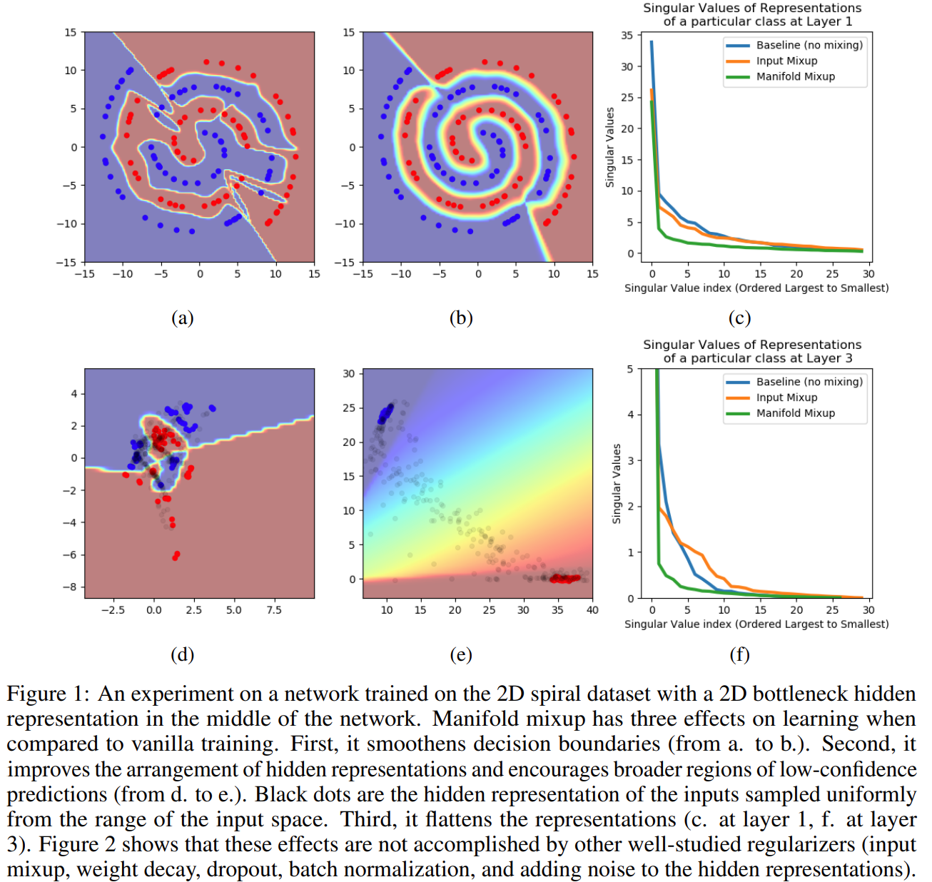
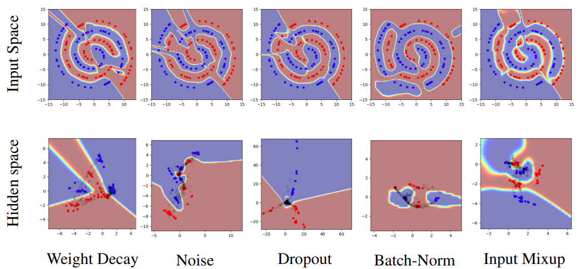
Manifold Mixup improves the hidden representations and decision boundaries of neural networks at multiple layers.
PatchUp: a hidden state block-level regularization technique, which is applied on selected contiguous blocks of feature maps from a random pair of samples.
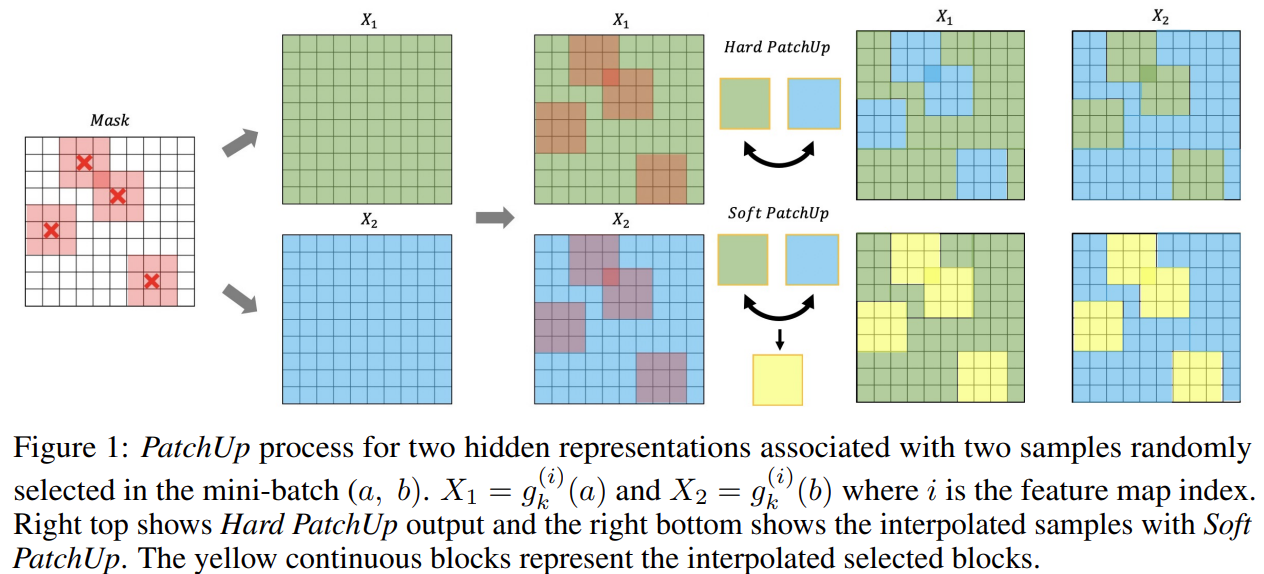
PatchUp could be seen as CutMix on Manifold of hidden states.
PuzzleMix: exploit saliency and local statistics for optimal mixup.
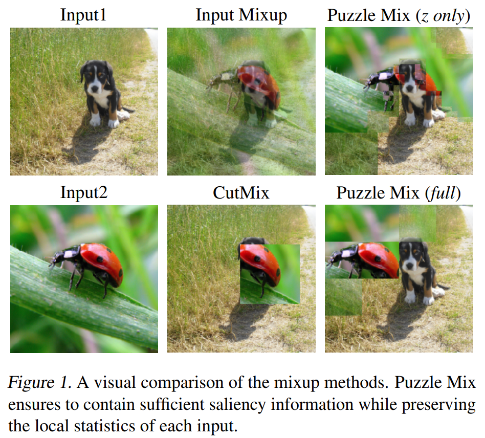
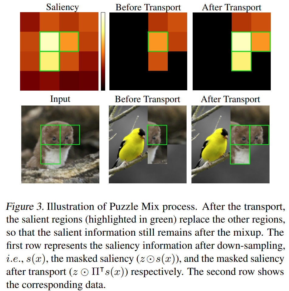
Randomly selecting mask is not a proper strategy because it may mask some regions with important information (objects). PuzzleMix utilizes the saliency to avoid this problem.
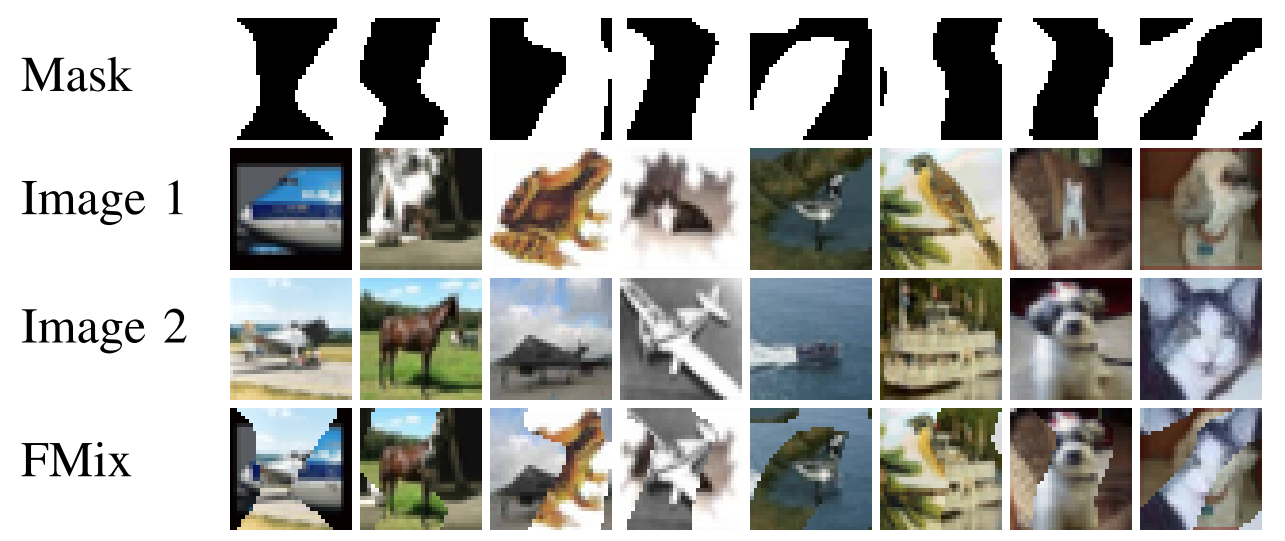
FMix: include masks of arbitrary shape rather than just square. It samples a low frequency grey-scale mask from Fourier space which can then be converted to binary with a threshold.