CoST

PAPER: CoST: Contrastive Learning of Disentangled Seasonal-Trend Representations for Time Series Forecasting

Motivations

Previous work of time series representation learning is mainly focusing on three aspects as follows:

Reduce complexity (sparse attention) of Transformer for long sequence modeling
Sample proper contrastive pairs
Find better paradigm of data augmentation

In fact, none of these approaches above truly leverages the structural information of time series. For example, recent work on video representation learning is trying to introduce structural priors (decouple video into context and motion) into training. Thus, an intuitive idea is to find structural information or invariant features of time series and take them as input.

Compared to video, image or even natural language, time series is more redundant. Jointly learning features end-to-end from observed data may lead to the model over-fitting and capturing spurious correlations of the unpredictable noise. Some existing methods formulate time series as a sum of trend, seasonal and error variables like follows:

$X$: observed data
$E$: unpredictable error/noise of $X$
$X^*$: error-free latent variable
$T,S$: trend and seasonal variable

CoST assumes that seasonal and trend modules do not influence or inform each other. Even if one mechanism changes due to a distribution shift, the other remains unchanged. That is to say, CoST supposes that trend and seasonality are more invariant and robust features, from which we can learn better representation of the raw data.

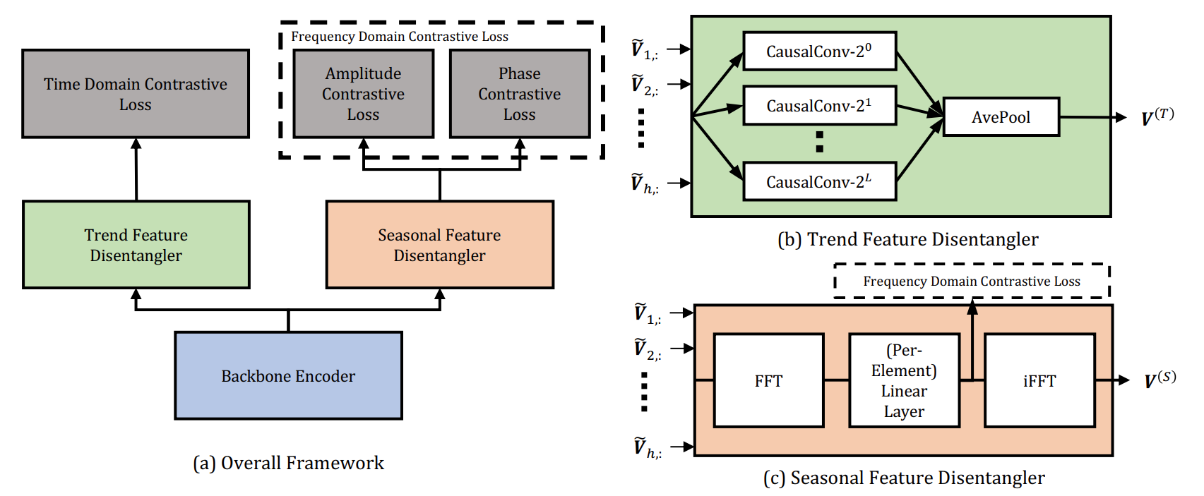
CoST takes casual TCN as its backbone encoder. Trend representations are learned in the time domain while seasonal representations are learned via frequency domain.

TFD: a mixture of CasualConv with the look-back windows of different size and a pooling layer
SFD: a learnable Fourier layer

Both TFD and SFD are optimized by contrastive loss. Different views are augmented by scaling, shifting and jittering.

Positive samples: the different views of the same data
Negative samples: the same view of different data in the same mini-batch

\[L=L_{\text{time}}+\frac{\alpha}{2}(L_{\text{amp}}+L_{\text{phase}})\]

Notice that CoST applies a dynamic dictionary like MoCo to save negative samples. To avoid coping with complex number in SFD, CoST directly uses amplitude and phase to capture representation in frequency domain.

Experiments

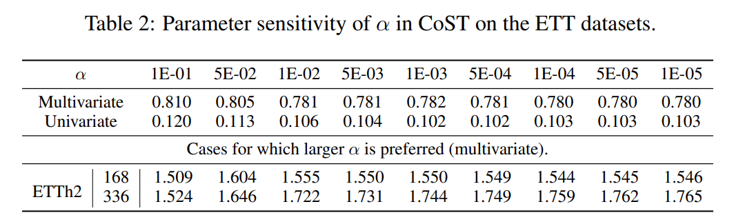
Sensitivity analysis shows that the seasonal component has lower importance than the trend component in most cases. In other experiments, CoST takes $\alpha$ as 5e-4.

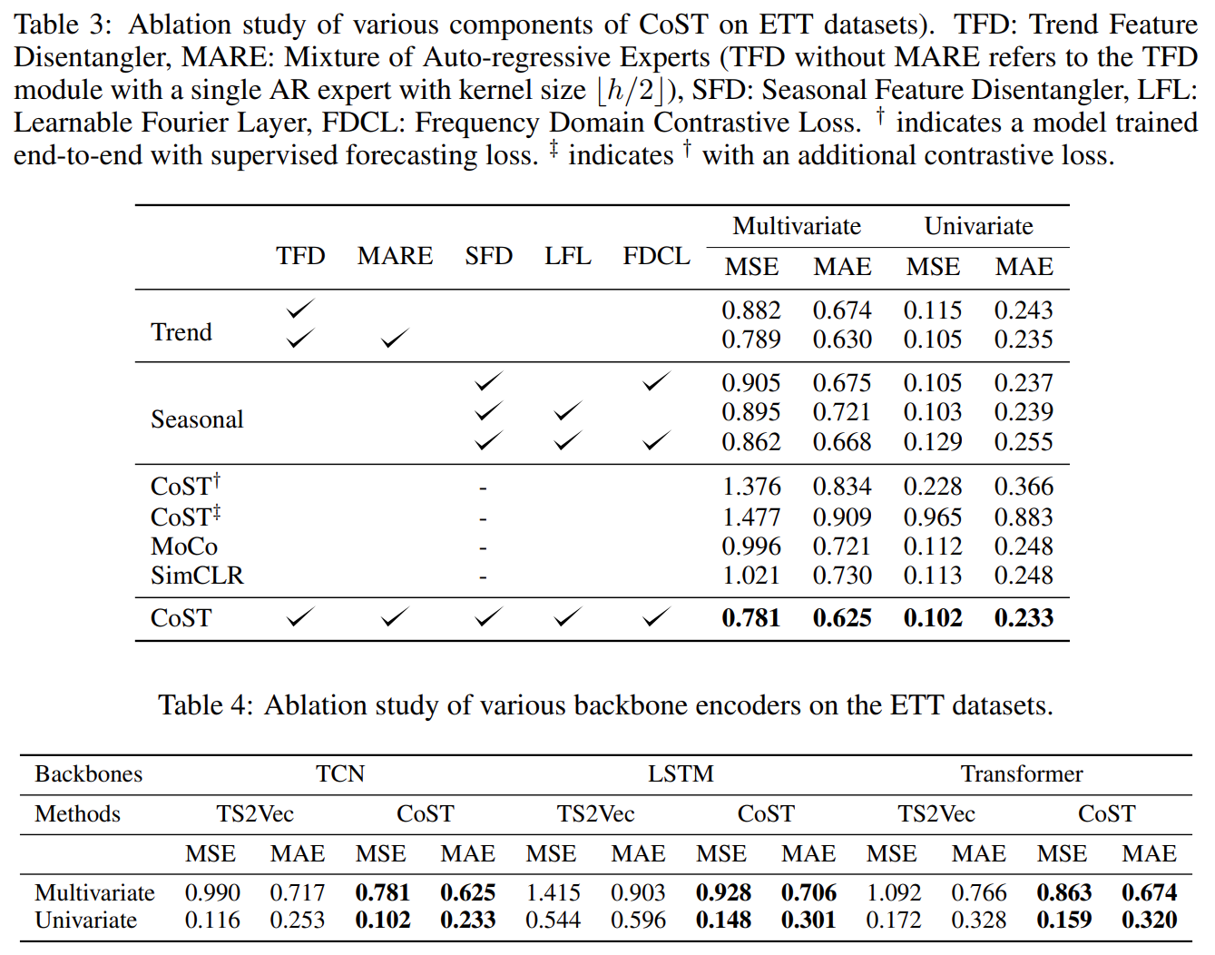
Ablation study shows the effect of all the components in CoST. TFD means they just use a single AR expert. Up to now, Transformer-based model is not better than existing methods in classification and forecasting tasks.

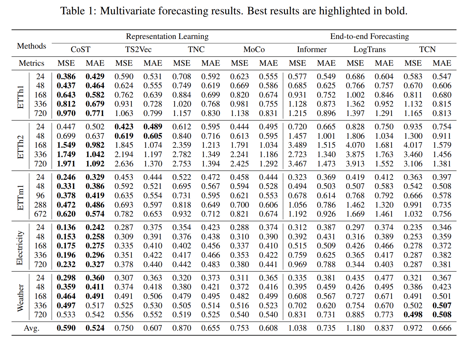
Compared to TS2Vec

TS2Vec and CoST are both contrastive representation learning approaches. They have tried different data augmentation methods and hierarchical tricks:

	TS2Vec	CoST
Mainly task	classification	forecasting
Data augmentation	clip	scale, shift and jitter
Hierarchical	pooling features in optimization	multi-scale extractor like FPN

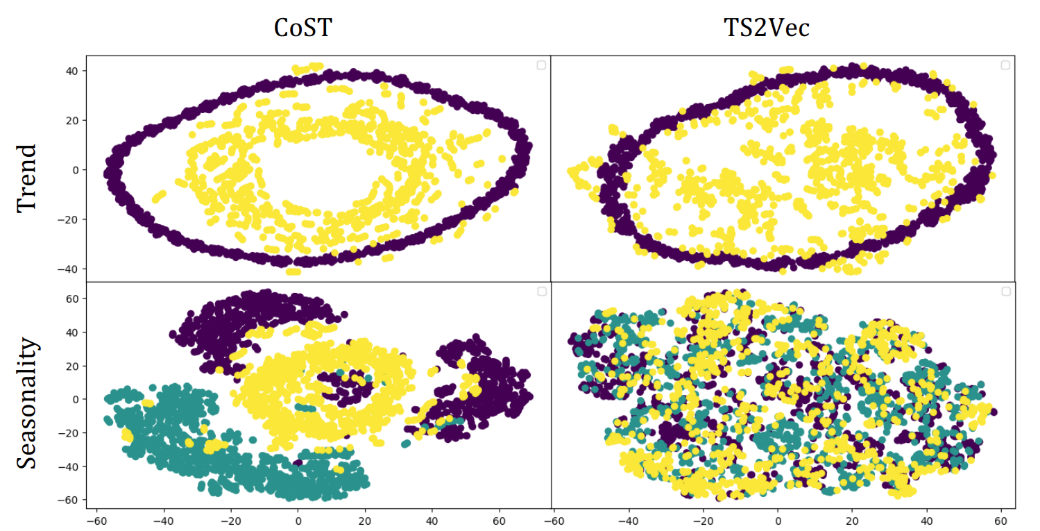
Apparently, CoST is better than TS2Vec due to introducing new structural priors in frequency domain. But we still need more experiments to compare the effect of different data augmentation and different hierarchical tricks. (e.g. DilatedConv)