Introduction
- Why: Self-supervised learning empowers us to exploit a variety of labels that come with the data for free.
- Aim: Learn intermediate representation that can carry good semantic or structural meanings from series of auxiliary tasks (always accompany with data augmentation) and can be beneficial to a variety of practical downstream tasks.

The three keys to learn a good representation in self-supervised learning are mentioned above. Choose a good feature extractor and find proper auxiliary tasks. Then optimize your loss/goal with respect to these auxiliary tasks.
For example, BERT is widely used in language modeling. It takes attention as feature extractor and is trained with two auxiliary tasks as follows:
- Mask language model: Randomly mask $15\%$ of tokens in each sequence, then predict the missing words.
- Next sentence prediction: Motivated by the fact that many downstream tasks involve the understanding of relationships between sentences, BERT samples sentence pairs and tells whether one sentence is the next sentence of the other.
Image-Based
A common workflow is to train a model on auxiliary tasks with unlabelled images and then use one intermediate feature layer of this model to feed a multinomial logistic regression classifier on ImageNet classification. The final classification accuracy quantifies how good the learned representation is. Here are some auxiliary tasks used in previous works.
Distortion (Transformation)
The auxiliary task is to discriminate between a set of distorted images. (e.g. translation, rotation, scaling, etc.)
Small distortion expectantly does not modify original semantic meaning or geometric forms of images. Slightly distorted images are considered the same as original and thus, the learned features are expected to be invariant to distortion. In Exemplar-CNN, all the distorted patches from the same patch should be classified into the same class in the auxiliary task.
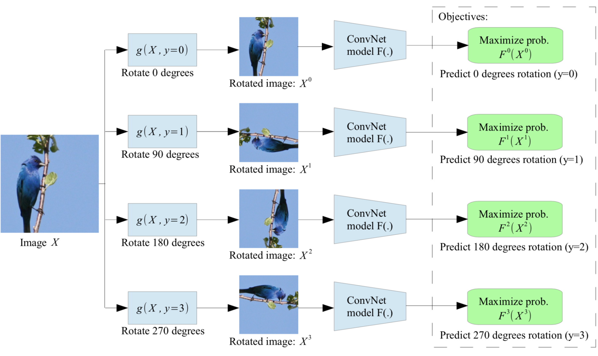
Rotation offers a cheap way of distortion. The auxiliary task is to predict which rotation has been applied, which is a 4-class classification problem.
Patches
The auxiliary task is to predict the relationship between multiple patches extracted from one image.
Context Prediction formulates a pretext task as predicting the relative position between two random patches from one image. Randomly sample the first patch and sample the second patch from its $8$ neighboring locations. The model is trained to predict where the second patch is.
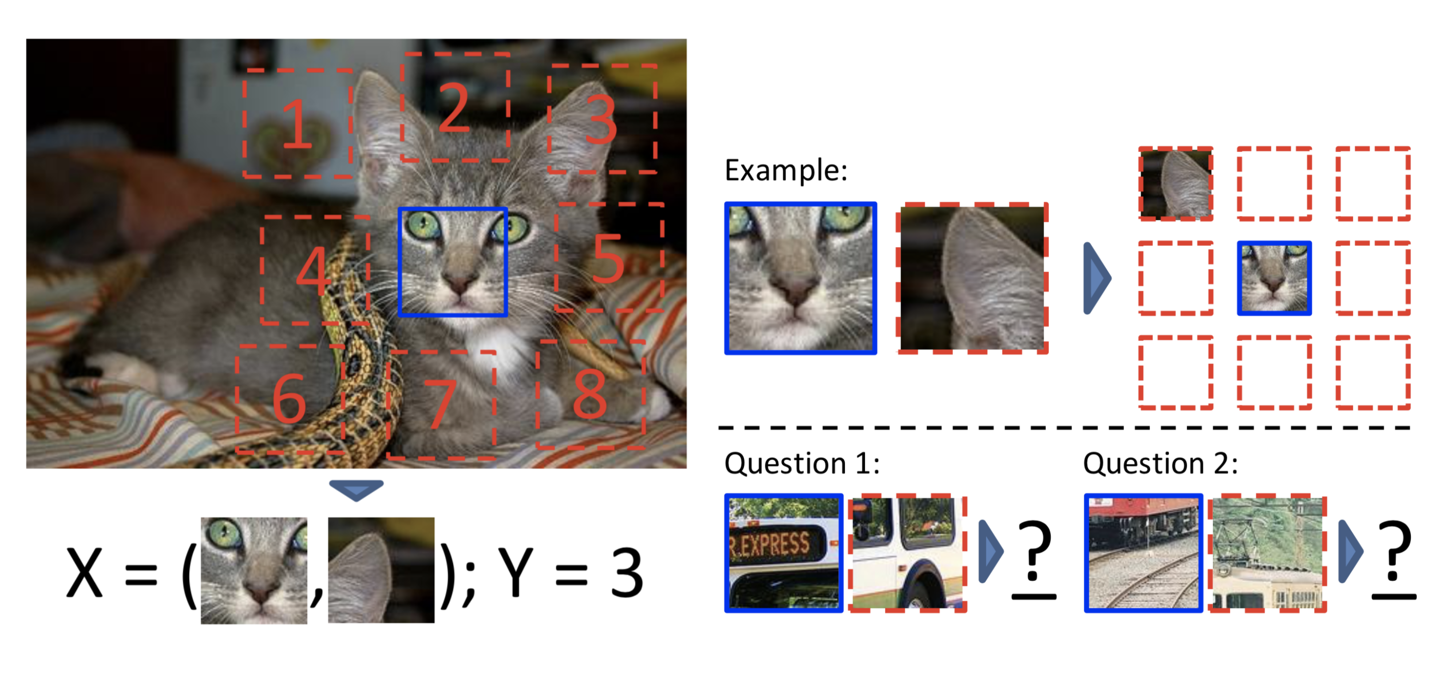
To avoid the model only catching low-level trivial signals, such as connecting a straight line across boundary or matching local patterns, we need additional noise to avert these shortcuts.
- Add gaps between patches
- Randomly downsample some patches and then upsampling it
- Randomly drop $2$ of $3$ color channels (chromatic aberration)
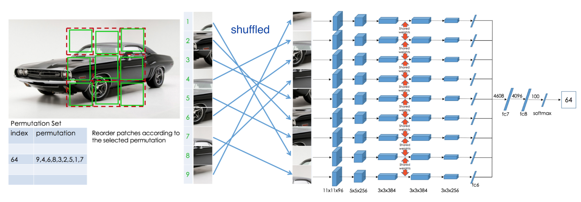
Based on $3\times3$ grid in each image, jigsaw puzzle game is proposed as auxiliary task: place $9$ shuffled patches back to the original locations.
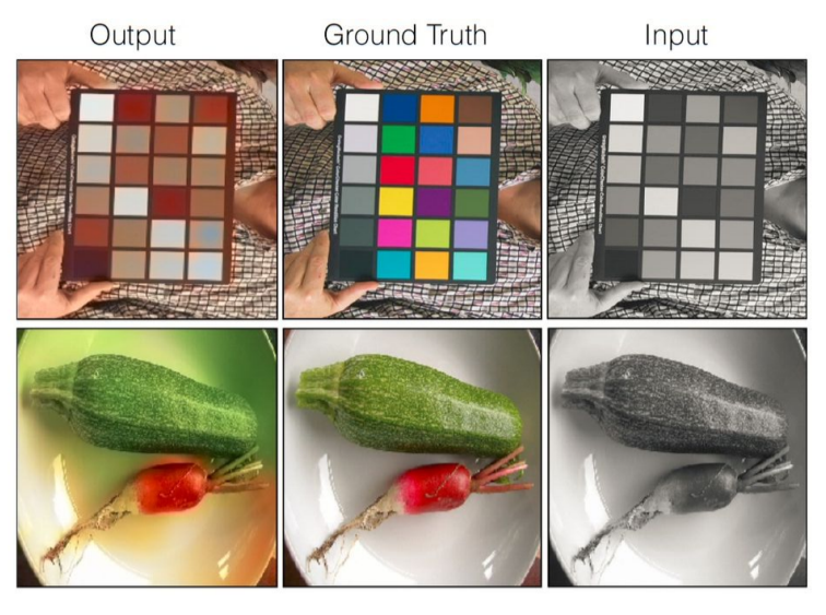
Colorization
The auxiliary task is to color a grayscale input image. Colorization concerns about how to generate vibrant and realistic images. Thus, it is a good way of data augmentation.
Generative Modeling
The auxiliary task is to reconstruct the original input (sometimes with noise or missing piece) while learning meaningful latent representation.
Context Encoders is trained to fill in a missing piece in the image. It’s a pity that there was no feature extractor as powerful as transformer at that time. And they were too conservative in the use of masks.
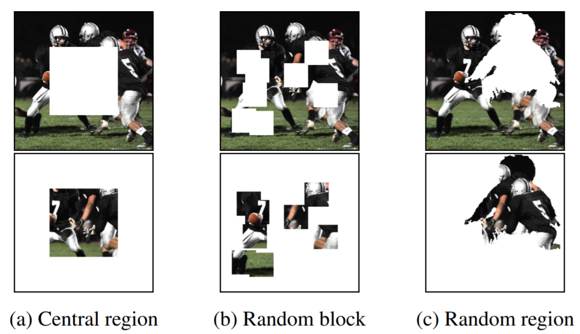
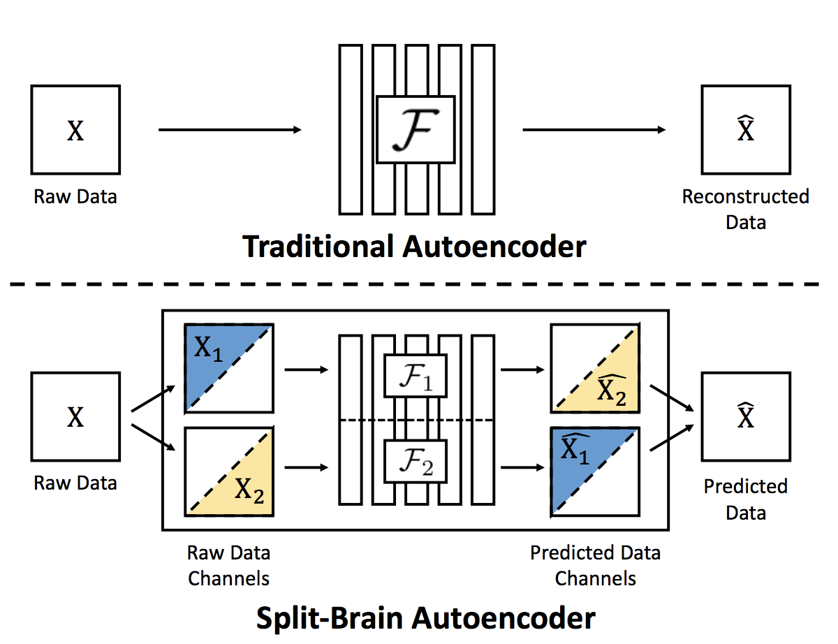
The problem of traditional cross-channel encoder is that only part of the data is used for feature extraction and another as the prediction or reconstruction target. In case of colorization, the model can only extract features from the grayscale image and is blind to color, leaving the color information unused. When applying a mask on an image, the context encoder removes information of all the color channels in partial regions which is also not used in feature extraction.
The split-brain autoencoder is trained to do two complementary predictions with some known information. In this paper, it trys to predict a subset of color channels from the rest of channels. Split-brain encoder successfully utilizes all the information of the raw data. It can be seen as aggregation of multiple autoencoders.
Other generative models like generative adversarial networks (GANs) are also able to capture semantic information from the data. Due to space reasons, I will not show here for the time being.
Up to now, ViT has proven that transformer is better in feature extraction than CNN because it can take into account both short-range and long-range dependence issues. Based on ViT, MAE has improved performance of predicting masked patches.
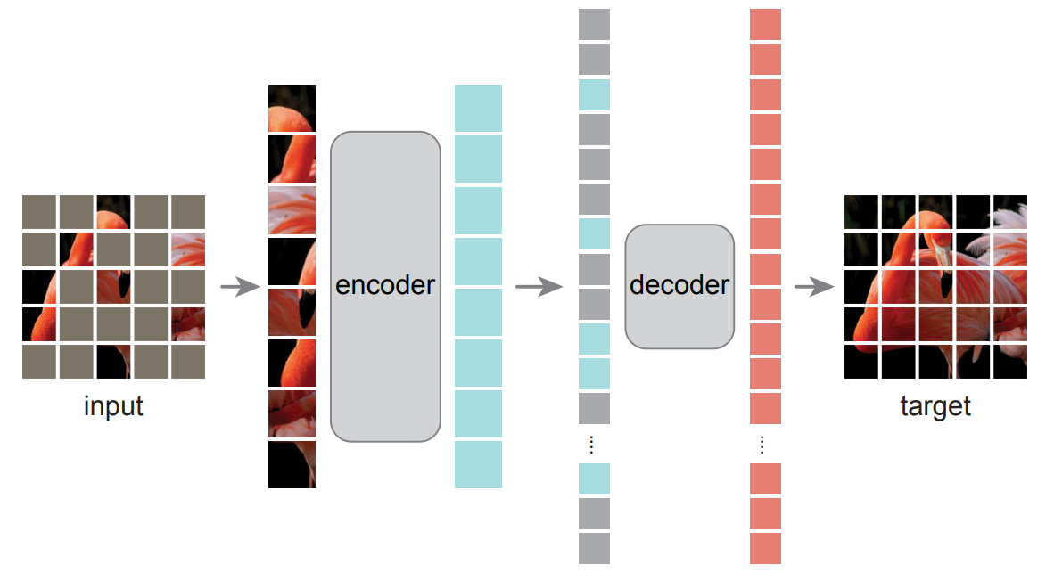
The key insights of MAE are as follows. You can see more details in original paper or here.
- High ratio of mask usage
- Randomly mask patches for each iteration
- Remove mask token from the encoder
- Lightweight decoder which reconstructs image on pixel level
Video-Based
A video contains a sequence of semantically related frames. The order of frames describes certain rules of reasonings and physical logics. Here are some auxiliary tasks used in previous works.
Tracking
The auxiliary task is to track moving objects in videos to learn good representation of each frame. Two patches connected by a track should have similar visual representation in deep feature space. To avoid the model learn to map everything to the same value, Siamese Triplet Network adds negative samples into training.
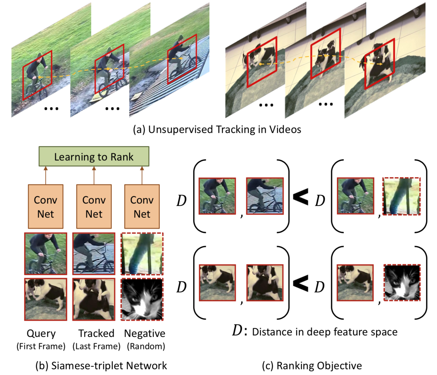
Notice the positive patches can be selected by optical flow. The negative patches come from the same batch in training. In this paper, they have tried to do hard negative mining to find top-k negative samples.
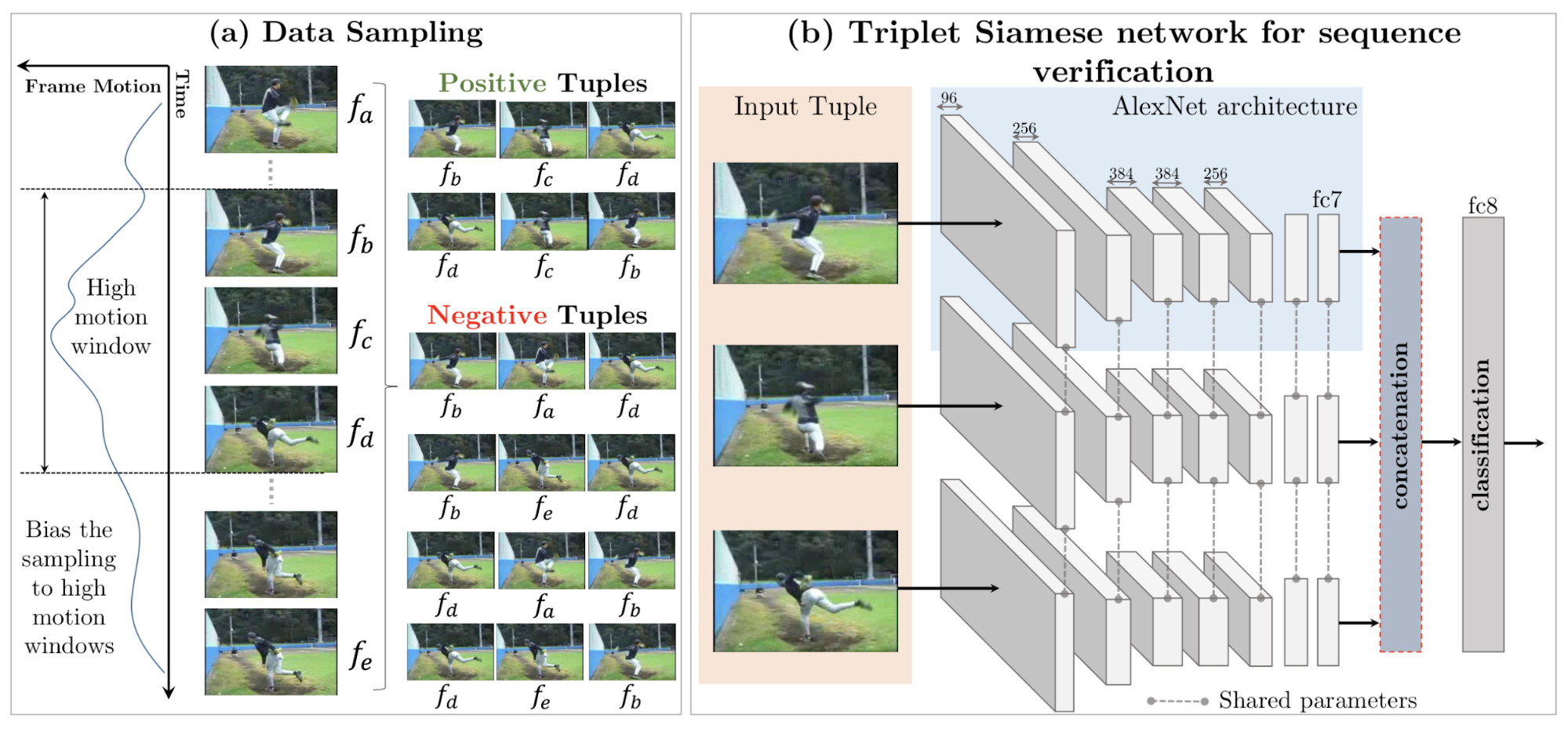
Frame Sequence
The auxiliary task is to validate frame order or predict the arrow of time. The training frames are sampled from high-motion windows. Positive samples are consecutive frames and negative samples are in error order. The model is trained to determine whether a sequence of frames is placed in the correct temporal order.
Video Colorization
The auxiliary task is to copy colors from a normal reference frame in color to another target frame in grayscale by leveraging the natural temporal coherency of colors across video frames.
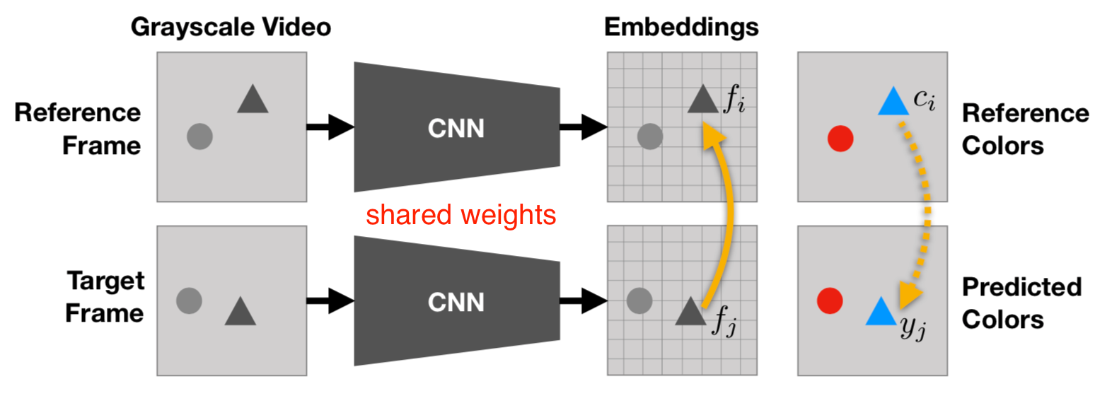
The model takes two neighboring grayscale frames as input. Using softmax similarity, the model points from the target frame into the reference frame embeddings and then copies the color back into the predicted frame. It works well when downstream task is about video segmentation.
Contrastive Learning
The goal of contrastive representation learning is to learn such an embedding space in which similar sample pairs stay close to each other while dissimilar ones are far apart. (To some extent similar to metric learning.) Key ingredients are as follows:
- Heavy Data Augmentation: It introduces the non-essential variations into examples without modifying semantic meanings.
- Large Batch Size: It guarantees that loss function can cover adequate negative samples. (A trick: Memory Bank)
- Hard Negative Mining: It’s important to find a good way of negative sampling.
Contrastive Loss (2005)
Contrastive loss takes a pair of inputs $(x_i,x_j)$ and minimizes the embedding distance when they are from the same class but maximizes the distance otherwise.
\[L(x_i,x_j,\theta)=\mathbb{I}_{y_i=y_j}\|f_\theta(x_i)-f_\theta(x_j)\|^2+\mathbb{I}_{y_i\not=y_j}\max(0,\varepsilon-\|f_\theta(x_i)-f_\theta(x_j)\|)^2\]$\varepsilon$ is a hyperparameter, defining the lower bound distance between samples of different classes.
Triplet Loss (2015)
Given one anchor input $x$, we select one positive sample $x^+$ and one negative sample $x^-$. Triplet loss learns to minimize the distance between $x$ and $x^+$ and maximize the distance between $x$ and $x^-$ at the same time.
\[L(x,x^+,x^-)=\sum_{x\in X}\max(0,\|f(x)-f(x^+)\|^2-\|f(x)-f(x^-)\|^2+\varepsilon)\]The margin parameter $\varepsilon$ is configured as the minimum offset between distances of similar vs dissimilar pairs.
Lifted Structured Loss (2015)
Lifted structured loss utilizes all the pairwise edges within one training batch for better computational efficiency.
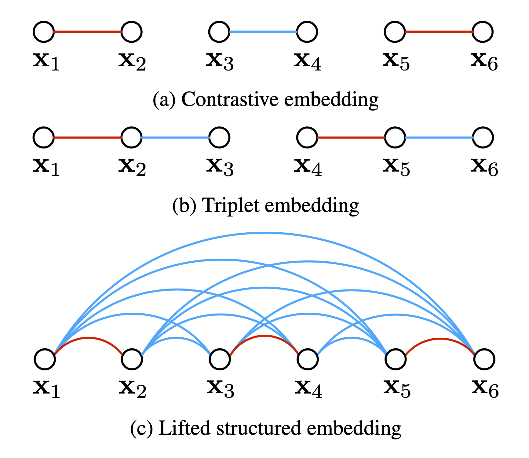
Let $D_{ij}=|f(x_i)-f(x_j)|^2$, then:
\[L=\frac{1}{2\vert P\vert}\sum_{(i,j)\in P}\max(0,L_{ij})^2\] \[L_{ij}=D_{ij}+\max(\max_{(i,k)\in N}(\varepsilon-D_{ik}),\max_{(j,l)\in N}(\varepsilon-D_{jl}))\]$P$ contains the set of positive pairs and $N$ is the set of negative pairs. $L_{ij}$ is used for mining hard negatives.
N-pair Loss (2016)
N-pair loss generalizes triplet loss to include comparison with multiple negative samples.
\[\begin{aligned} L(x,x^+,\{x_i^-\}_{i=1}^{N-1}) &=\log(1+\sum_{i=1}^{N-1}\exp(f(x)^Tf(x_i^-)-f(x)^Tf(x^+))) \\ &=-\log\frac{\exp(f(x)^Tf(x^+))}{\exp(f(x)^Tf(x^+))+\sum_{i=1}^{N-1}\exp(f(x)^Tf(x^-_i))} \end{aligned}\]If we only sample one negative sample per class, it is equivalent to the softmax loss for multi-class classification.
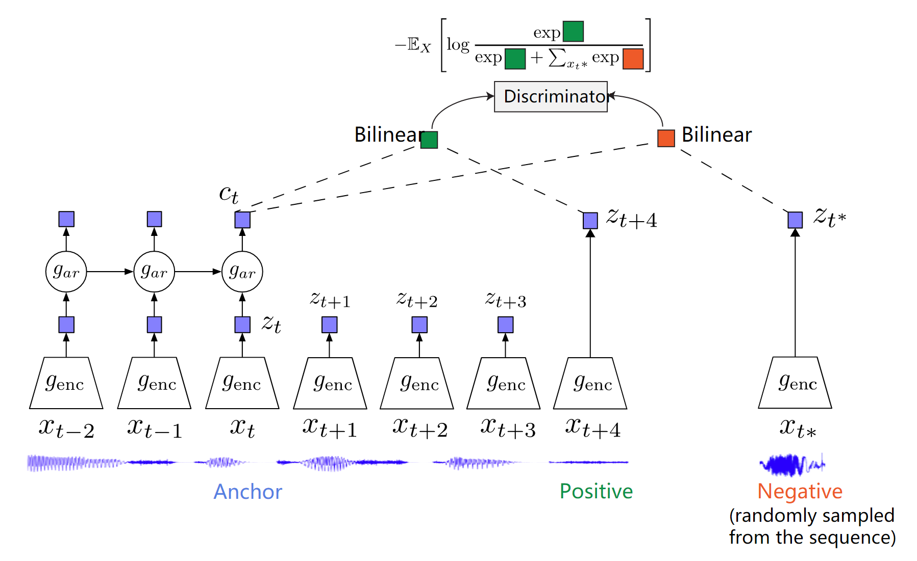
InfoNCE (2018)
Representation Learning with Contrastive Predictive Coding