图像频域滤波处理

前导
理想滤波
高斯滤波
巴特沃斯滤波

图像频域分析

读取图像

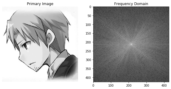
  使用 opencv 读取灰度图,利用 numpy.fft.fft2 对二维灰度图进行快速傅里叶变换,将图像从空间域转换为频域;再对频域图进行 numpy.fft.fftshift 移频,将图像中的低频部分移动到图像中心便于可视化;再取频谱的绝对值得到幅度谱,利用 np.log() 进行对数变换以提高低灰度区域的对比度,使原本频谱图中的较暗像素得到增强,最后绘制原始图像和处理后的频域图形。整个流程的完整代码如下:

1
2
3
4
5
6
7
8
9
img = cv2.imread('image/lls.png', 0) # 读取灰度图
f = np.fft.fft2(img) # 空间域 -> 频域
fshift = np.fft.fftshift(f) # 移频
s = np.log(np.abs(fshift)) # 对数变化幅频
# 绘制图像
plt.figure(figsize=(10, 10))
plt.subplot(121), plt.imshow(img, 'gray'), plt.axis("off"), plt.title('Primary Image')
plt.subplot(122), plt.imshow(s, 'gray'), plt.title('Frequency Domain')
plt.show()

image_processing_1_0.png

滤波处理

理想低通滤波器

  理想低通滤波器的公式如下:

\[H(u, v)=\begin{cases}1, & D(u, v)\le D_0 \\ 0, & D(u, v)>D_0\end{cases}\]

ideal_low.png

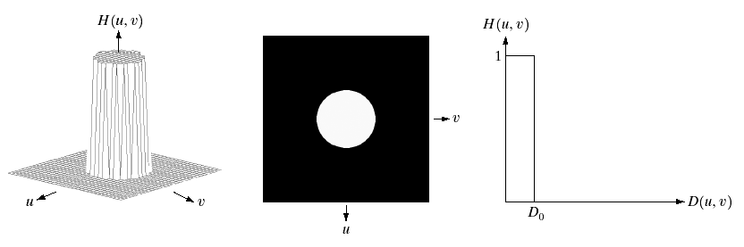
  其中 $D(u, v)$ 为频率域上点 $(u, v)$ 到中心 $(r_0, c_0)$ 的距离,$D_0$ 为截止频率。实验中我们取 $D$ 为欧氏距离,即 $D(u ,v)=\sqrt{(u-r_0)^2+(v-c_0)^2}$

1
2
3
def cal_distance(pa, pb):
    dis = sqrt((pa[0]-pb[0])**2 + (pa[1]-pb[1])**2)
    return dis

  对于所有滤波器的构造,我们均使用掩膜(mask)处理的方法,即构造一个与原频谱矩阵尺寸相同的掩膜,选择保留的部分设为 1,不保留的部分设为 0,对掩膜和原频谱矩阵做哈达玛积(Hadamard product)即可实现过滤效果,得到滤波后的频谱图,再进行频移和傅里叶反变换即可得到滤波后图像。完整的理想低通滤波器代码如下:

1
2
3
4
5
6
7
8
9
10
11
12
13
14
15
16
17
18
19
20
21
22
23
24
25
26
'''
    @param image: 原始图像
    @param S: 原始图像的标准化幅频
    @param d: 截止频率
    @return new_img: 滤波后图像
    @return fshift*d_matrix: 滤波后频谱
'''
def lowPassFilter(image, S, d):
    f = np.fft.fft2(image)
    fshift = np.fft.fftshift(f)
    # 滤波处理
    def make_transform_matrix(d):
        transfor_matrix = np.zeros(image.shape)
        center_point = tuple(map(lambda x:(x-1)/2, S.shape))
        for i in range(transfor_matrix.shape[0]):
            for j in range(transfor_matrix.shape[1]):
                dis = cal_distance(center_point,(i,j))
                if dis <= d:
                    transfor_matrix[i,j]=1
                else:
                    transfor_matrix[i,j]=0 # 过滤高频分量
        return transfor_matrix
    d_matrix = make_transform_matrix(d)
    # 傅里叶反变换
    new_img = np.abs(np.fft.ifft2(np.fft.ifftshift(fshift*d_matrix)))
    return new_img, fshift*d_matrix

  实验中我们选取 $D_0=20$ 和 $D_0=80$ 两种截止频率的理想低通滤波器,滤波后的图像和频谱图如下:

1
2
3
4
img1, fshift1 = lowPassFilter(img, s, 20)
s1 = np.log(np.abs(fshift1))
img2, fshift2 = lowPassFilter(img, s, 80)
s2 = np.log(np.abs(fshift2))

image_processing_4_0.png

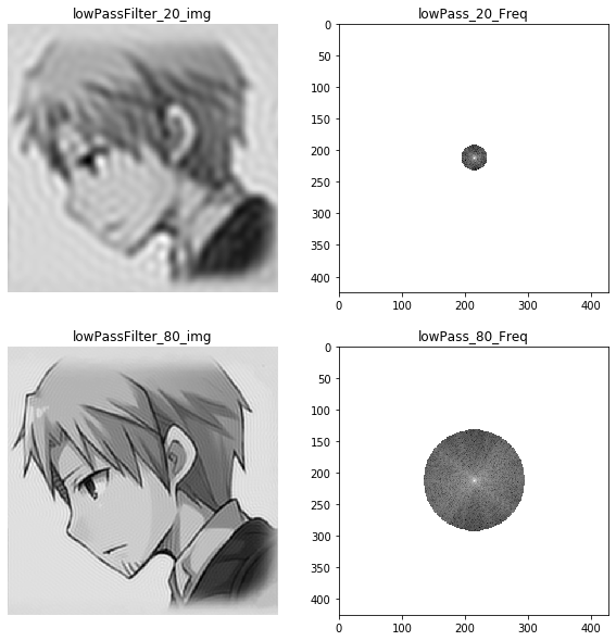
  可以看出,图像的低频成分对应图像变化缓慢的部分,即图像大致的相貌和轮廓。低通滤波器起到图像模糊/平滑的作用,截止频率较小时图像会变得很模糊;截止频率较大时图像会变得稍微清晰。此外,由于理想低通滤波器直接过滤了所有的高频分量,频谱的变化存在一个急剧的过度,这就会产生振铃现象(图像中类似于波纹一样的成分),截止频率越小,振铃现象越明显。

理想高通滤波器

  理想高通滤波器的公式如下:

\[H(u, v)=\begin{cases}0, & D(u, v)\le D_0 \\ 1, & D(u, v)>D_0\end{cases}\]

  理想高通滤波器与理想低通滤波器刚好相反,其参数含义与之相同,我们同样使用掩膜的方法直接过滤频谱图中的低频分量。完整的理想高通滤波器代码如下:

1
2
3
4
5
6
7
8
9
10
11
12
13
14
15
16
17
18
19
def highPassFilter(image, S, d):
    f = np.fft.fft2(image)
    fshift = np.fft.fftshift(f)
    # 滤波处理 
    def make_transform_matrix(d):
        transfor_matrix = np.zeros(image.shape)
        center_point = tuple(map(lambda x:(x-1)/2, S.shape))
        for i in range(transfor_matrix.shape[0]):
            for j in range(transfor_matrix.shape[1]):
                dis = cal_distance(center_point,(i,j))
                if dis <= d:
                    transfor_matrix[i,j]=0 # 过滤低频分量
                else:
                    transfor_matrix[i,j]=1
        return transfor_matrix
    d_matrix = make_transform_matrix(d)
    # 傅里叶反变换
    new_img = np.abs(np.fft.ifft2(np.fft.ifftshift(fshift*d_matrix)))
    return new_img, fshift*d_matrix

  实验中我们选取 $D_0=20$ 和 $D_0=80$ 两种截止频率的理想高通滤波器,滤波后的图像和频谱图如下:

1
2
3
4
img3, fshift3 = highPassFilter(img, s, 20)
s3 = np.log(np.abs(fshift3))
img4, fshift4 = highPassFilter(img, s, 80)
s4 = np.log(np.abs(fshift4))

image_processing_7_0.png

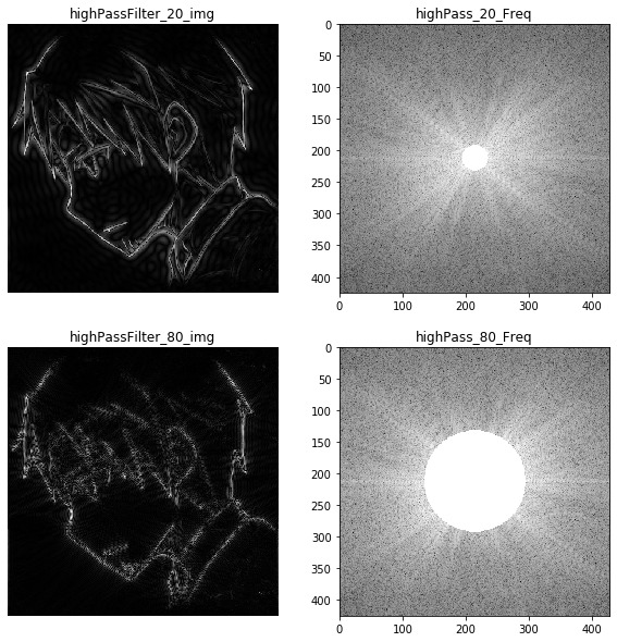
  可以看出,图像的高频成分对应图像变化迅速的部分,即图像中的边缘部分,表明了图像中目标边缘的强度及方向。高通滤波器起到图像锐化的作用,截止频率较小时对边缘的刻画越明显;截止频率较大时则变得稍微模糊。与理想低通滤波器相似,由于频谱中存在急剧的过度,同样会产生振铃现象,截止频率越小,振铃现象越明显。

高斯低通滤波器

  高斯低通滤波器的公式如下:

\[H(u, v)=\exp({\frac{-D^2(u, v)}{2D_0^2}})\]

gaussian_low.png

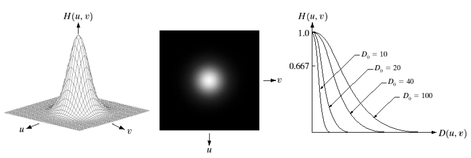
  不同于理想低通滤波器直接舍去高频分量的做法,高斯滤波是根据高斯分布函数的形状决定局部像素的权值,从而对整个频谱图的每个像素进行加权处理(同样通过掩膜实现),这就使得频谱的变化是连续的,不存在突变的情况。完整的高斯低通滤波器代码如下:

1
2
3
4
5
6
7
8
9
10
11
12
13
14
15
16
def GaussianLowFilter(image, S, d):
    f = np.fft.fft2(image)
    fshift = np.fft.fftshift(f)
    # 滤波处理
    def make_transform_matrix(d):
        transfor_matrix = np.zeros(image.shape)
        center_point = tuple(map(lambda x:(x-1)/2, S.shape))
        for i in range(transfor_matrix.shape[0]):
            for j in range(transfor_matrix.shape[1]):
                dis = cal_distance(center_point,(i,j))
                transfor_matrix[i,j] = np.exp(-(dis**2)/(2*(d**2))) # 加权
        return transfor_matrix
    d_matrix = make_transform_matrix(d)
    # 傅里叶反变换
    new_img = np.abs(np.fft.ifft2(np.fft.ifftshift(fshift*d_matrix)))
    return new_img, fshift*d_matrix

  实验中我们选取 $D_0=20$ 和 $D_0=80$ 两种截止频率的高斯低通滤波器,滤波后的图像和频谱图如下:

1
2
3
4
img7, fshift7 = GaussianLowFilter(img, s, 20)
s7 = np.log(np.abs(fshift7))
img8, fshift8 = GaussianLowFilter(img, s, 80)
s8 = np.log(np.abs(fshift8))

image_processing_13_0.png

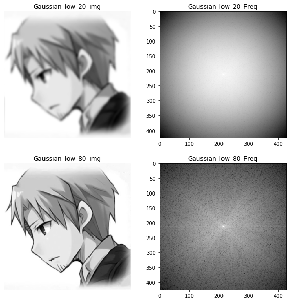
  可以看出,高斯低通滤波器的过度特性非常平坦,滤波后的图像不会产生明显的振铃现象,其清晰程度相较于理想低通滤波器有了很大的提升。

高斯高通滤波器

  高斯高通滤波器的公式如下:

\[H(u, v)=1-\exp({\frac{-D^2(u, v)}{2D_0^2}})\]

  与高斯低通滤波器相同,高斯高通滤波器同样根据高斯分布函数对频谱图中的每个像素进行加权处理使得频谱图的变化连续。完整的高斯高通滤波器代码如下:

1
2
3
4
5
6
7
8
9
10
11
12
13
14
15
16
def GaussianHighFilter(image, S, d):
    f = np.fft.fft2(image)
    fshift = np.fft.fftshift(f)
    # 滤波处理
    def make_transform_matrix(d):
        transfor_matrix = np.zeros(image.shape)
        center_point = tuple(map(lambda x:(x-1)/2, S.shape))
        for i in range(transfor_matrix.shape[0]):
            for j in range(transfor_matrix.shape[1]):
                dis = cal_distance(center_point,(i,j))
                transfor_matrix[i,j] = 1-np.exp(-(dis**2)/(2*(d**2))) # 加权
        return transfor_matrix
    d_matrix = make_transform_matrix(d)
    # 傅里叶反变换
    new_img = np.abs(np.fft.ifft2(np.fft.ifftshift(fshift*d_matrix)))
    return new_img, fshift*d_matrix

  实验中我们选取 $D_0=20$ 和 $D_0=80$ 两种截止频率的高斯高通滤波器,滤波后的图像和频谱图如下:

1
2
3
4
img5, fshift5 = GaussianHighFilter(img, s, 20)
s5 = np.log(np.abs(fshift5))
img6, fshift6 = GaussianHighFilter(img, s, 80)
s6 = np.log(np.abs(fshift6))

image_processing_10_0.png

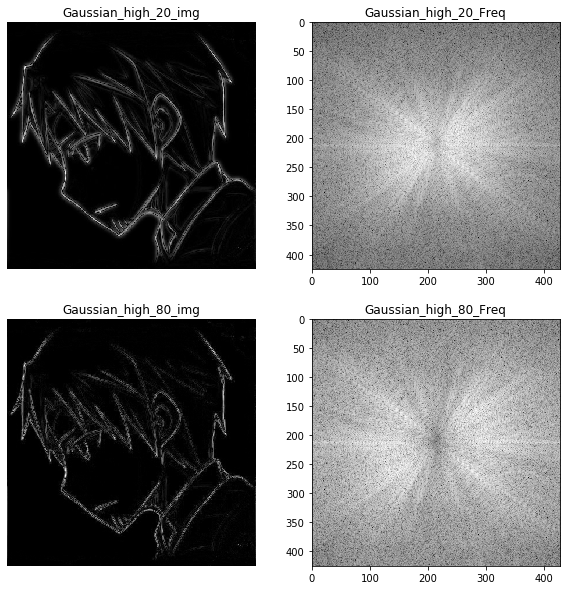
  与理想高通滤波器相比,由于经过高斯高通滤波器后的频谱图变化仍是连续的,在保留原始图像边缘轮廓的同时,也不存在明显的振铃现象,轮廓的细节和清晰度相较于理想高通滤波器都有了很大的提升。

巴特沃斯低通滤波器

  巴特沃斯低通滤波器的公式如下:

\[H(u, v)=\frac{1}{1+(D(u, v)/D_0)^{2n}}\]

butter_low.png

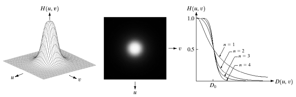
  巴特沃斯滤波的处理思路与高斯滤波相似,选取漏斗形函数对频谱图的每个像素进行加权处理以实现频谱的连续化,其频率响应曲线十分平滑。不同的是巴特沃斯滤波引入了阶数 $n$ 来控制曲线收敛到 $0$ 的速度。完整的巴特沃斯低通滤波器代码如下:

1
2
3
4
5
6
7
8
9
10
11
12
13
14
15
16
def butterworthLowPassFilter(image, S, d ,n):
    f = np.fft.fft2(image)
    fshift = np.fft.fftshift(f)
    # 滤波处理
    def make_transform_matrix(d):
        transfor_matrix = np.zeros(image.shape)
        center_point = tuple(map(lambda x:(x-1)/2, S.shape))
        for i in range(transfor_matrix.shape[0]):
            for j in range(transfor_matrix.shape[1]):
                dis = cal_distance(center_point,(i,j))
                transfor_matrix[i,j] = 1/((1+(dis/d))**n) # 加权
        return transfor_matrix
    d_matrix = make_transform_matrix(d)
    # 傅里叶反变换
    new_img = np.abs(np.fft.ifft2(np.fft.ifftshift(fshift*d_matrix)))
    return new_img, fshift*d_matrix

  实验中我们选取 $D_0=20, n=1$、$D_0=80, n=1$、$D_0=20, n=4$ 和 $D_0=80, n=4$ 四种不同截止频率和阶数的巴特沃斯低通滤波器,滤波后的图像和频谱图如下:

1
2
3
4
5
6
7
8
img13, fshift13 = butterworthLowPassFilter(img, s, 20, 1)
s13 = np.log(np.abs(fshift13))
img14, fshift14 = butterworthLowPassFilter(img, s, 80, 1)
s14 = np.log(np.abs(fshift14))
img15, fshift15 = butterworthLowPassFilter(img, s, 20, 4)
s15 = np.log(np.abs(fshift15))
img16, fshift16 = butterworthLowPassFilter(img, s, 80, 4)
s16 = np.log(np.abs(fshift16))

image_processing_20_0.png

image_processing_21_0.png

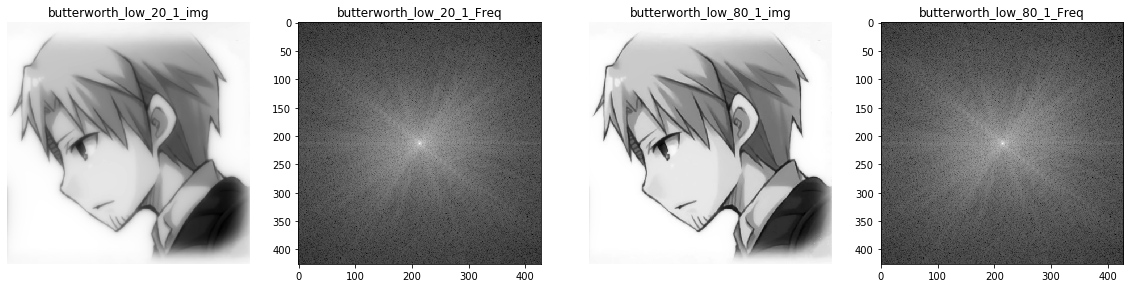
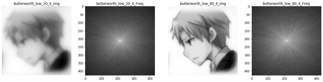
  可以看出,当阶数较高时,巴特沃斯低通滤波的表现接近于理想低通滤波;当阶数较低时表现接近于高斯低通滤波。阶数越大,曲线收敛速度越快,滤波后图像里的振铃现象越为明显。

巴特沃斯高通滤波器

  巴特沃斯高通滤波器的公式如下:

\[H(u, v)=\frac{1}{1+(D_0/D(u, v))^{2n}}\]

  与巴特沃斯低通滤波器相似,同样是引入阶数 $n$ 的漏斗形函数。完整的巴特沃斯高通滤波器代码如下:

1
2
3
4
5
6
7
8
9
10
11
12
13
14
15
16
def butterworthHighPassFilter(image, S, d ,n):
    f = np.fft.fft2(image)
    fshift = np.fft.fftshift(f)
    # 滤波处理
    def make_transform_matrix(d):
        transfor_matrix = np.zeros(image.shape)
        center_point = tuple(map(lambda x:(x-1)/2, S.shape))
        for i in range(transfor_matrix.shape[0]):
            for j in range(transfor_matrix.shape[1]):
                dis = cal_distance(center_point,(i,j))
                transfor_matrix[i,j] = 1/((1+(d/dis))**n) # 加权
        return transfor_matrix
    d_matrix = make_transform_matrix(d)
    # 傅里叶反变换
    new_img = np.abs(np.fft.ifft2(np.fft.ifftshift(fshift*d_matrix)))
    return new_img, fshift*d_matrix

  实验中我们选取 $D_0=20, n=1$、$D_0=80, n=1$、$D_0=20, n=4$ 和 $D_0=80, n=4$ 四种不同截止频率和阶数的巴特沃斯高通滤波器,滤波后的图像和频谱图如下:

1
2
3
4
5
6
7
8
img9, fshift9 = butterworthHighPassFilter(img, s, 20, 1)
s9 = np.log(np.abs(fshift9))
img10, fshift10 = butterworthHighPassFilter(img, s, 80, 1)
s10 = np.log(np.abs(fshift10))
img11, fshift11 = butterworthHighPassFilter(img, s, 20, 4)
s11 = np.log(np.abs(fshift11))
img12, fshift12 = butterworthHighPassFilter(img, s, 80, 4)
s12 = np.log(np.abs(fshift12))

image_processing_16_0.png

image_processing_17_0.png

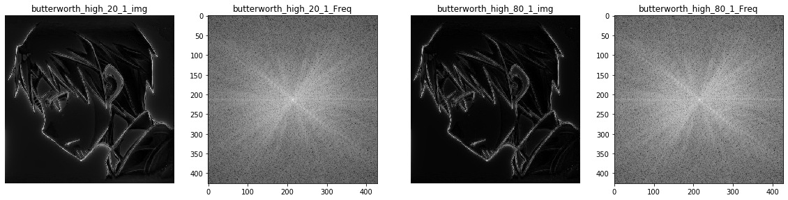
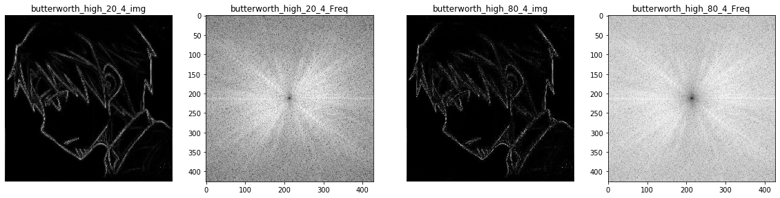
  可以看出,当阶数较高时,巴特沃斯高通滤波的表现接近于理想高通滤波;当阶数较低时表现接近于高斯高通滤波。阶数越大,曲线收敛速度越快,滤波后图像里的振铃现象越为明显。